Lesson 6
| Site: | MoodleHUB.ca 🍁 |
| Course: | Math 20-1 SS |
| Book: | Lesson 6 |
| Printed by: | Guest user |
| Date: | Thursday, 4 December 2025, 2:15 AM |
Description
Created by IMSreader
1. Lesson 6
Module 4: Quadratic Equations and Inequalities
Lesson 6: Solving Systems of Equations Algebraically
Focus

The World’s Fair of 1893 was an opportunity for the city of Chicago, Illinois, to showcase its architecture, technology, and the spirit of America. When the architects and designers were charged with the task of bringing the vision of a world’s fair to life, they were faced with the challenge of outdoing the World Exhibition of 1889, held in Paris to commemorate the centennial of the French Revolution. The Eiffel Tower was the centrepiece of the World Exhibition. Standing at 300 m, it became the undisputed tallest structure in the world, dwarfing the Washington Monument by twice the size.
In order to “out-Eiffel Eiffel,” and also to attract as many visitors as possible, the architects designed a lavish city within a city with magnificent buildings, exquisitely manicured landscapes, and the world’s first Ferris wheel. While the Ferris wheel did not rival the Eiffel tower in terms of height, reaching only 80.4 m (or approximately 27 storeys), the Ferris wheel was commanding in its own right. With a total of 36 cars, each of which could accommodate 60 people, the Ferris wheel could handle 2160 passengers!
The design and construction of an attractive and entertaining fairground depends to a great extent on mathematics. Mathematics is used in the design of rides, such as a rollercoaster or a Ferris wheel, and in impressive shows, such as a choreographed water show or fireworks.
In this lesson you will continue to investigate linear-quadratic and quadratic-quadratic systems. You will learn how to solve these types of systems algebraically. You will use methods that are similar to those that you have previously studied.
Outcomes
At the end of this lesson you will be able to
- determine and verify the solution of a system of linear-quadratic or quadratic-quadratic equations algebraically
- solve a problem that involves a system of linear-quadratic or quadratic-quadratic equations and explain the strategy used
- model a situation using a system of linear-quadratic or quadratic-quadratic equations
Lesson Questions
You will investigate the following questions:
- Why do systems of equations yield the correct solutions even after they have been manipulated algebraically?
- Why is it important to be able to solve systems of equations algebraically as well as graphically?
Assessment
Your assessment may be based on a combination of the following tasks:
- completion of the Lesson 6 Assignment (Download the Lesson 6 Assignment and save it in your course folder now.)
- course folder submissions from Try This and Share activities
- additions to Module 4 Glossary Terms and Formula Sheet
- work under Project Connection
1.1. Launch
Module 4: Quadratic Equations and Inequalities
Launch
Do you have the background knowledge and skills you need to complete this lesson successfully? This section, which includes Are You Ready? and Refresher, will help you find out.
Before beginning this lesson you should be able to
- solve systems of linear equations by substitution and by elimination
- apply the Pythagorean theorem
1.2. Are You Ready?
Module 4: Quadratic Equations and Inequalities
Are You Ready?
Complete these questions. If you experience difficulty and need help, visit Refresher or contact your teacher.
- Solve the following systems of equations by substitution.
- Solve the following systems of equations by elimination.
- State the Pythagorean theorem. Answer
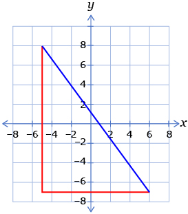
- Use the Pythagorean theorem to determine the length of the hypotenuse of the triangle shown. Assume that each grid square is equal to one unit. Answer
1.3. Refresher
Module 4: Quadratic Equations and Inequalities
Refresher
Use the following to review the topics you experienced difficulties with in the Are You Ready? section.
Use the Solving Linear Systems Algebraically series of interactive lessons. Complete the following lessons:
- Solving Systems by Substitution
- Solving Systems by Elimination (Addition or Subtraction)
You may also want to try the last two lessons, which deal with applications and strategy selection.

Use Pythagorean Theorem to review the definition of this important theorem in mathematics. The demonstration applet gives a visual representation of the theorem.
Go back to the Are You Ready? section and try the questions again. If you are still having difficulty, contact your teacher.
1.4. Discover
Module 4: Quadratic Equations and Inequalities
Discover
Try This 1
Consider this system of equations comprised of two functions:
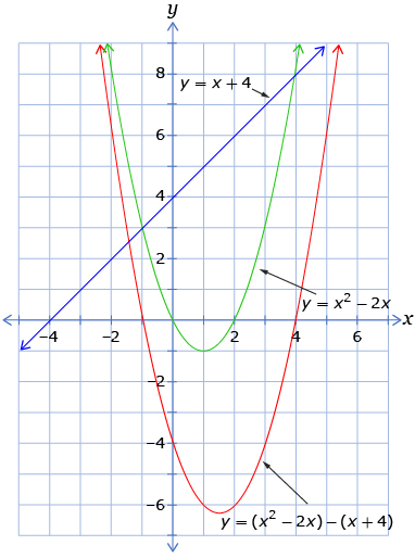
y = x2 − 2x
y = x + 4
- Construct a table like the following. Leave room for a fourth column as shown. Fill in the y-coordinates corresponding to the given x-coordinates for each of the functions. The first two rows have been completed as an example.
x y = x2 − 2x y = x + 4 −3 15 1 −2 8 2 −1 0 1 2 3 4 5
- Use the table to create a graph. Plot the coordinates of the two functions. Join the points of each function with a smooth curve or line.
- Show where the solutions to the system of equations are on the graph.
- Label the last column of your chart “Difference of Equations.” In this column, evaluate the difference between the y-coordinates of the first two equations. For example, the difference in the first row would be recorded (15 − 1) or 14, and the difference in the second row would be (8 − 2) = 6.
x y = x2 − 2x y = x + 4 Difference of Equations −3 15 1 14 −2 8 2 6 −1 0 1 2 3 4 5
- Plot the points made from the coordinates of the x-values in the first column and the y-values from the final column. Join the points with a smooth curve. You may wish to use a different colour from the first two functions.
You may want to work together with a partner to complete the Analysis questions.
Analysis
- How could you determine the x-values of the solutions to the system of equations by looking only at the graph of the third function? Circle the x-values of the solutions on the graph.
- Write the equation representing the difference of the two equations. How can you use this equation to algebraically determine the solution to the system of equations?

- What if you reversed the order of the subtraction and evaluated the other difference? How would your third graph change? Would you still be able to use that graph to determine the solutions to the system?
![]() Save your work in your course folder.
Save your work in your course folder.
Share 1
In Try This 1 you worked through steps to find the solution to a system of equations. You subtracted the two equations to find the difference between them and then graphed this difference to find the solutions. You then found the solutions algebraically. Working with a classmate, discuss the following questions based on your Try This 1 observations. Then write a short paragraph that summarizes the answers.
- How did the solutions found using the graph compare to the solutions found algebraically?
- Did the order in which you subtracted the equations have an effect on the solutions?
- Both graphing the difference and finding the difference algebraically help you to find the x-values of the solutions. What then should be your next step?
![]() Save your work in your course folder.
Save your work in your course folder.
You will investigate algebraic methods of solving systems of equations in the remainder of the lesson. You may want to refer to your Try This 1 investigation as you explore the concepts presented.
1.5. Explore
Module 4: Quadratic Equations and Inequalities
Explore

© Looby-Lou/1555394/Fotolia
In an animated fountain, water streams reach different heights and may also take on different colours. A musical fountain is an extension of this concept: the movement of the streams is synchronized with upbeat music. The Fountains of Bellagio in Las Vegas, Nevada, have the power to shoot streams of water up to 24 storeys high, and, at any given point during a show, there could be up to 65 000 L of water in the air! The water show has been choreographed to music by a variety of different artists, such as Elvis Presley, Céline Dion, the Mormon Tabernacle Choir, and Luciano Pavarotti.
In this lesson you will solve systems of linear-quadratic and quadratic-quadratic equations algebraically. Later in the lesson you will model a situation related to a musical fountain using a system of equations.
1.6. Explore 2
Module 4: Quadratic Equations and Inequalities
Solving Linear Equations Algebraically
Recall from your previous studies two algebraic methods used to solve a system of linear equations.
The following chart summarizes the main idea of each method.
| Substitution | Elimination |
| Rearrange one of the equations for a single variable. Substitute the expression for the variable into the other equation. | Multiply the equations by constants such that the coefficients of the x-terms or the y-terms either match or have a sum of zero. |
Try This 2
Consider the following linear-quadratic system.
y = −x2 + 3
x + 2y = 6
- Solve the system by substitution.
- Solve the system by elimination.
- Verify your solutions. You may choose to do this by substituting the determined values into the original equations or by graphing.
![]() Save your work in your course folder.
Save your work in your course folder.
Share 2
There are four main ways of solving the system of equations from Try This 2—two variations each of substitution and elimination.
- Compare your solutions from Try This 2 with a partner. Between the two of you, complete a table like the one shown by copying the appropriate solutions into the appropriate columns.
Substitution:
Isolate ySubstitution:
Isolate xElimination:
Eliminate yElimination:
Eliminate x
- For any solutions that are not covered by either your work or your partner’s work, consider together how you would solve the system by the method indicated. Then record your solutions in the appropriate columns.
- Discuss which method(s) you prefer and give reasons why. Under what circumstances would you use some of the other methods that you did not prefer for the system in Try This 2?
![]() Save your work in your course folder.
Save your work in your course folder.
1.7. Explore 3
Module 4: Quadratic Equations and Inequalities
Choosing a Solution Strategy
Turn to “Example 1” on pages 441 to 442 of the textbook. Without looking at the solution, try to solve the system on your own.
Two methods are presented as possible solution strategies: substitution and elimination. From Try This 2, you know that there are different approaches you can take within each of these methods. Work through the solution shown in the textbook. As you do so, focus on these questions:
- What reason is given for the solution strategy? For example, why is a particular variable selected for isolating or eliminating over the other variable?
- For the substitution method, how do you know which equation to substitute into once a variable is isolated?
- For the elimination method, which term is the target for elimination? Is it the squared term, the linear term, or the constant?
Self-Check 1
Complete Do You Know Your Linear-Quadratic Equations?
Using Differences to Solve Systems of Equations
Retrieve your work from Try This 1.
In that activity, you learned that you can also solve the system by graphing the difference of the equations.
y = x2 − 2x
y = x + 4
Compare your answer to Analysis question 7 to the following:
Look at your answer to Try This 1, Analysis question 6. Your graphs may look like the following.

Watch Graphing the Difference.
So, from an algebraic perspective, you must also be able to determine the solutions to the system by determining the roots of the difference of the equations. In this case, you could determine the roots of the equation x2 − 3x − 4 = 0. This can be done by any of several algebraic methods, such as factoring, square root strategies, or the quadratic formula.
Does this same idea apply to systems of quadratic-quadratic equations? You will find out in Try This 3.
1.8. Explore 4
Module 4: Quadratic Equations and Inequalities
Try This 3
- Consider the following quadratic-quadratic system.
y = 3x2 + x − 2
y = x2 + 2x + 1
Solve this system algebraically by following this example shown for the linear-quadratic system:
- Reduce the system to a single equation in one variable using elimination.
- Determine the solution(s) algebraically to the resulting equation using an appropriate strategy.
- Verify your solution(s) algebraically.
- Reduce the system to a single equation in one variable using elimination.
![]() Save your work in your course folder.
Save your work in your course folder.
Share 3
- Compare your solution strategies with a partner. Discuss the relative advantages and drawbacks of the strategies for
- reducing the system to a single equation
- solving the quadratic equation
- reducing the system to a single equation
- Why is it difficult to solve this system by eliminating the x-variable instead of the y-variable?
-
- With your partner, manipulate the system so that you can eliminate the x2-term. Graph the resulting equation, as well as the equations in the system.
y = 3x2 + x − 2
y = x2 + 2x + 1
- What do you notice about graphing the equations from part a?
- With your partner, manipulate the system so that you can eliminate the x2-term. Graph the resulting equation, as well as the equations in the system.
- How can a strategy for solving the original system be developed based on your observations from question 3?
![]() Save your work in your course folder.
Save your work in your course folder.
Self-Check 2
Complete questions 3.d., 4.d., 5.a., and 7 on pages 451 and 452 in the textbook. Answer

Hemera/Thinkstock
1.9. Explore 5
Module 4: Quadratic Equations and Inequalities
Using Algebra to Solve Problems Modelled by Systems Involving Quadratic Equations
In the previous lesson you modelled problems with systems of linear-quadratic equations and quadratic-quadratic equations. You solved those problems graphically. In the final section of this lesson, you will continue to develop your skills in modelling problems with systems. You will, however, focus on solving the problems algebraically.
Try This 4

Heritage Days Fesitval, Hawrelak Park photo (Edmonton: www.girlsandbicycles.ca, Sarah Chan, 2010.) Reproduced with permission.
The August long weekend in Edmonton always marks the celebration of Heritage Festival. The annual event showcases the food, culture, and wares of many countries, ranging from Afghanistan to Zimbabwe. In preparation for the event, approximately 65 pavilions are raised all over the 150-ac Hawrelak Park.
Assume that some of the pavilions in Hawrelak Park are arranged in the shape of a parabola, as shown in the following diagram.
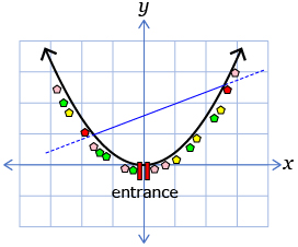
The parabola is described by the equation y = 0.003x2 + 0.005x. A path described by the equation y = 0.08x + 105 connects two food ticket kiosks, which are represented by red pentagons in the diagram. In both cases, x represents the horizontal distance (in metres) from the entrance and y represents the vertical distance (in metres) from the entrance.
- Determine the coordinates of the two kiosks.
- What is the length of the path between the two kiosks?
![]() Save your work in your course folder.
Save your work in your course folder.
You will need to retrieve your work later in the lesson for review with a partner.
1.10. Explore 6
Module 4: Quadratic Equations and Inequalities
Modelling a Problem with a System of Two Quadratic Equations
Try This 5
Launch Modelling Quadratic-Quadratic Equations: Animated Fountain. Work through the example to model and solve a problem based on a system of quadratic-quadratic equations. You will be given a lot of support to model the problem. Once you have the system set up, you will have the opportunity to solve the system independently based on the strategies you have learned in this lesson. Then complete the following question. Note: You will copy your answer to this question into your Lesson 6 Assignment later in the lesson.
In an animated fountain, a stream of water is shot to a maximum height of 10 ft and re-enters the fountain 6 ft away. A second stream of water is shot to a maximum height of 5 ft but re-enters the fountain 14 ft away. Each stream follows a parabolic path. At what horizontal distance from the water jets are the two streams at the same height?
Copy the system that you modelled in Modelling Quadratic-Quadratic Equations: Animated Fountain as part of your solution. Solve the system algebraically showing all of your work. You do not need to show how you obtained the equations.
![]() Save your work in your course folder.
Save your work in your course folder.
Self-Check 3
Complete questions 9, 13, 17, and 18 on pages 452 to 455 in the textbook. Answer
1.11. Connect
Module 4: Quadratic Equations and Inequalities
Open your copy of the Lesson 6 Assignment, which you saved in your course folder at the start of this lesson. Complete the assignment.
![]() Save your work in your course folder.
Save your work in your course folder.
Project Connection

© wong yu liang/29976438/Fotolia
Go to Module 4 Project: Imagineering. Complete Step 4: Marketing.
![]() Save your work in your course folder.
Save your work in your course folder.
Going Beyond
The following graph shows the parabola with equation y = x2. How can you use algebra to determine the values of the slope of a linear function that would intersect a given parabola in one, two, or zero points?
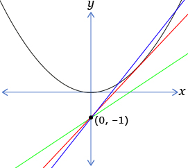
Consider the system of equations represented by the graph.
y = x2
y = mx − 1
Solve this system to determine the values of m that would result in
- two solutions
- one solution
- no solutions
You may have to use what you learned about the discriminant in Lesson 4 in order to complete this exercise. Some aspects of the solution will be covered in the final lesson of this module, so you may wish to return to this problem after completing the module.
![]() Save your work in your course folder.
Save your work in your course folder.
1.12. Lesson 6 Summary
Module 4: Quadratic Equations and Inequalities
Lesson 6 Summary

© Argus/17415175/Fotolia
In this lesson you investigated the following questions:
- Why do systems of equations yield the correct solutions even after they have been manipulated algebraically?
- Why is it important to be able to solve systems of equations algebraically as well as graphically?
You previously learned how to solve systems of linear-quadratic and quadratic-quadratic equations based on graphical methods. In this lesson you studied how to solve these systems using algebraic techniques. You used substitution and elimination strategies to manipulate the equations in each system. You learned that you can algebraically manipulate the equations in a system without changing the solutions. You verified this conclusion by graphing, as shown in the following graph from the Discover section of the lesson.

Knowing how to algebraically solve math problems, such as systems of equations, is an important skill for understanding math principles. While a graphical solution is often easy to obtain, such a solution process does not reveal the process by which the solution is obtained from a mathematical standpoint. Algebraic methods, when applied correctly, can take you step-by-step from problem to solution, which leads, in turn, to understanding and insight.
In the remaining lessons of this module, you will consider linear and quadratic inequalities, studying them from both a graphical and algebraic perspective.