Lesson 7
| Site: | MoodleHUB.ca 🍁 |
| Course: | Math 20-1 SS |
| Book: | Lesson 7 |
| Printed by: | Guest user |
| Date: | Thursday, 4 December 2025, 2:21 AM |
Description
Created by IMSreader
1. Lesson 7
Module 4: Quadratic Equations and Inequalities
Lesson 7: Graphing Linear and Quadratic Inequalities
Focus

© Heng kong Chen/492933/Fotolia
A popular concept amongst urban planners is the development of “cities within cities.” These developments are designed to be one-stop shopping destinations as well as recreation and entertainment centres. More than your typical shopping mall, these complexes include restaurants, hotels, business offices, and even residential space.
The city-within-a-city concept has been particularly popular in Asian countries. In some Asian countries, booming economies and increasing consumer and housing demand have driven architects and designers to create all-encompassing mega-complexes.
Mathematics can help architects design complexes that meet the needs of residents and consumers alike.
In this lesson you will learn how you can use linear and quadratic inequalities to represent multiple variables, much like an architect might use mathematics to guide the development of a project involving multiple factors.
Outcomes
At the end of this lesson you will be able to
- explain, using examples, how test points can be used to determine the solution region that satisfies an inequality
- explain, using examples, when a solid or broken line should be used in the solution for an inequality
- sketch, with or without technology, the graph of a linear or quadratic inequality
- solve a problem that involves a linear or quadratic inequality
Lesson Questions
You will investigate the following questions:
- How are the properties of linear and quadratic inequalities in two variables related to their graphs?
- How are linear and quadratic inequalities in two variables applied in design?
Assessment
Your assessment may be based on a combination of the following tasks:
- completion of the Lesson 7 Assignment (Download the Lesson 7 Assignment and save it in your course folder now.)
- course folder submissions from Math Lab, Try This, and Share activities
- additions to Module 4 Glossary Terms and Formula Sheet
- work under Project Connection
Materials
You will need a ruler and graph paper.
1.1. Launch
Module 4: Quadratic Equations and Inequalities
Launch
Do you have the background knowledge and skills you need to complete this lesson successfully? This section, which includes Are You Ready? and Refresher, will help you find out.
Before beginning this lesson you should be able to
- solve linear inequalities in one variable
- graph linear functions
- identify slope and intercepts of a linear function
- graph a quadratic function
1.2. Are You Ready?
Module 4: Quadratic Equations and Inequalities
Are You Ready?
Complete these questions. If you need help, visit Refresher or contact your teacher.
- Solve the following inequalities.
- For linear functions of the form y = mx + b, describe what m and b represent. Answer
- Complete a table like the following.
Function Slope, if Linear x-intercept y-intercept Sketch 
3x + 2y + 8 = 0 y = 2x2 − 3x + 5
Answer
How did the questions go? If you feel comfortable with the concepts covered in the questions, skip forward to Discover. If you experienced difficulties, use the resources in Refresher to review these important concepts before continuing through the lesson.
1.3. Refresher
Module 4: Quadratic Equations and Inequalities
Refresher

Use the Inequality definition and applet to review the inequality symbols, the graphs of inequalities in one variable, and solving inequalities.

Use Graphing y = mx + b to review how to graph linear functions in the form y = mx + b. Select Linear Functions, and then select Graphing Equations in the Form y = mx + b on Graph Paper.
Refresh your skills in graphing a quadratic function.
- Return to Module 3: Lesson 3 to review how to convert a quadratic function in standard form to vertex form by completing the square.
- Use Quadratic Function (Vertex Form) to review the graphs of quadratic functions in the vertex form.

Go back to the Are You Ready? section and try the questions again. If you are still having difficulty, contact your teacher.
1.4. Discover
Module 4: Quadratic Equations and Inequalities
Discover

AbleStock.com/Thinkstock
In this Discover section you will begin to explore how you can graph linear and quadratic inequalities in two variables.
Try This 1
Part A: Linear Inequalities

Screenshot reprinted with permission of ExploreLearning
Launch Linear Inequalities in Two Variables - Activity A, and then follow the steps below. Record your responses as you work through the steps.
Step 1: Graph a linear function by adjusting the sliders for m and b. Notice that the line divides the coordinate plane into two areas. Record the linear function you graphed.
Step 2: Choose the “≤” symbol. How does the graph change?
Step 3: Select “Show solution test.” A blue point appears on the coordinate plane. What are the coordinates of the point? Does the test show this point as a solution to the inequality? On which side of the line does the point appear?
Step 4: Now drag the point to another part of the coordinate plane. Is this new point a solution to the inequality?
Step 5: Continue to experiment with different points, lines, and inequalities.
Analysis
- How would you describe the location of the points that are solutions to the inequality?
- A graph of a linear function would be only a straight line. Why do you think a shaded region is included in the graph of a linear inequality?
- How does the graph of the line change when you change the inequality symbol from ≤ or ≥ to < or >?
- What happens if you drag the point onto a dashed line? Is the point a solution? Likewise, what happens if you drag the point onto a solid line? Is the point a solution?
- How would you instruct someone to sketch y > x + 3?
- Describe the relationship between the inequality symbol of an inequality and the relative position of the shaded area on the corresponding graph.
Part B: Quadratic Inequalities

Screenshot reprinted with permission of ExploreLearning
Launch Quadratic Inequalities in Two Variables - Activity A. Use your observations from Quadratic Inequalities in Two Variables to add to or revise your responses to Analysis questions 1 to 6. Then complete question 7.
- What differences, if any, are there between linear inequalities and quadratic inequalities?
![]() Save your responses in your course folder.
Save your responses in your course folder.
You will revisit these results in Explore.
1.5. Explore
Module 4: Quadratic Equations and Inequalities
Explore

© Steven Holl Architects
The Linked Hybrid development is a twenty-first century housing complex located in Beijing, China. The complex is built on more than 15 ac (acres) of land and consists of over two million square feet dedicated to residential and commercial living spaces, entertainment and dining venues, underground parking, and even a kindergarten. This complex is truly a city within a city!
The design and construction of Linked Hybrid is an undertaking that requires consideration of a number of different factors. These factors are known as constraints. Constraints set limits, or boundaries, on what can be developed. Examples of constraints might be the space that is available for construction, the cost of materials and labour, and environmental considerations.
In this lesson you will explore linear and quadratic inequalities. You will learn how to use these inequalities to model situations involving constraints. You will explore multiple ways of graphing inequalities in two variables, with and without technology.
1.6. Explore 2
Module 4: Quadratic Equations and Inequalities
Forms of Linear and Quadratic Inequalities
Linear and quadratic inequalities come in different forms. The following table summarizes the four different forms of each kind of inequality.
Linear Inequalities in Two Variables (a, b, and c are real numbers) |
Quadratic Inequalities in Two Variables (a, b, and c are real numbers and a ≠ 0 ) |
| ax + by < c | y < ax2 + bx + c |
| ax + by ≤ c | y ≤ ax2 + bx + c |
| ax + by > c | y > ax2 + bx + c |
| ax + by ≥ c | y ≥ ax2 + bx + c |
An ordered pair (x, y) is considered a solution of an inequality if, when the values of x and y are substituted into the inequality, the inequality is true.
Try This 2
It is time to confirm the observations you made in Try This 1. You will focus on how the properties of linear and quadratic inequalities relate to their graphs.
Open Linear Inequalities in Two Variables - Activity A and Quadratic Inequalities in Two Variables - Activity A.

Screenshot reprinted with permission of ExploreLearning

Screenshot reprinted with permission of ExploreLearning
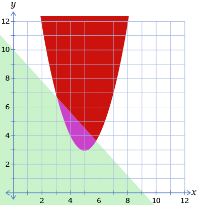
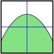
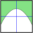
Consider the graphs shown.
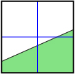
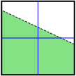

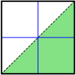
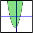

- For each graph, indicate whether the shaded region (in green) is above the boundary line or below the boundary line.
- For each graph, use either Linear Inequalities in Two Variables or Quadratic Inequalities in Two Variables to reconstruct the graph. Record the inequality you used to represent each graph.
![]() Save your response in your course folder.
Save your response in your course folder.
Share 1
Compare your results from Try This 2 with a partner. Note that you may not have the same inequalities for all, or any, of the graphs. However, you should have identical inequality symbols.
- Discuss or share any patterns you observed in both Try This 1 and Try This 2. These patterns may relate the inequality sign to
- the properties of the boundary lines
- the location of the shaded region
- the properties of the boundary lines
- Select a point on the boundary line of one of the inequalities. Then select a second point in the shaded region with the same x-coordinate as the point you previously selected. How do the y-coordinates of these two points compare to the inequality symbol used in the inequality?
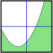
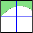
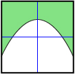
- Study the graph shown.

- Is the shaded region above or below the boundary line?
- How does this change the pattern for describing the shaded region?
- Is the shaded region above or below the boundary line?
![]() Save your response in your course folder.
Save your response in your course folder.
1.7. Explore 3
Module 4: Quadratic Equations and Inequalities
Graphing Inequalities in Two Variables

iStockphoto/Thinkstock
The graph of a linear inequality begins with the graph of a boundary line. The boundary line divides the coordinate plane into two separate regions, known as (open) half-planes. The boundary line is either dashed or solid, depending on whether the inequality permits points on the line to be included.
The half-plane that contains the points that satisfy the inequality is shaded. This set of points is known as the solution region.
Consider this strategy for graphing an inequality in two variables:
Step 1: Decide whether your boundary should be dashed or solid. If the inequality symbol is < or >, the boundary should be dashed. If the inequality symbol is ≤ or ≥, the boundary should be solid.
Step 2: Graph the boundary or the function corresponding to the inequality.
Step 3: Choose a point not on the boundary line. This is the test point.
Step 4: Check whether the test-point coordinates satisfy the inequality. If they do, shade the half-plane containing the point. If they don’t, shade the half-plane that does not contain the point.
Try This 3
Part A
- Graph the linear inequality 2x + 3y ≤ 6 using the steps in the strategy you just learned for graphing inequalities in two variables.
- Read part a. of “Example 1” and its solution on pages 466 and 467 of the textbook. This example is the same as question 1 above. Review both methods.
- Did you see the method you used in question 1 in the textbook solution?
- Which method do you prefer and why?
- Does your graph look the same as the one shown in the textbook?
- Did you see the method you used in question 1 in the textbook solution?
- Study part b. of “Example 1” on page 466. A possible method is presented for determining if a point is in the solution. Describe another method that can be used based on having a graph of the inequality.
Part B
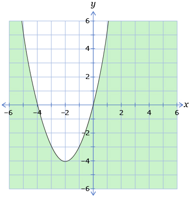
- Graph the quadratic inequality y ≥ x2 − 4x − 5 using the same steps as in Part A, question 1.
- Turn to “Example 2” on page 492 of the textbook. Compare the method presented in the textbook to the method you used.
- Answer the following questions based on your reading.
- Why would (−1, 0) be a poor choice for a test point?
- Besides the test-point method, what other method could you use to determine the proper half-plane to shade?
- Why would (−1, 0) be a poor choice for a test point?
![]() Save your responses in your course folder.
Save your responses in your course folder.
Self-Check 1
Launch Graphing Linear Inequalities. Work through pages 1 to 8 only. Read each section carefully before responding to the prompt.
1.8. Explore 4
Module 4: Quadratic Equations and Inequalities
Writing an Inequality to Describe a Given Graph
You have learned how to graph linear and quadratic inequalities in two variables. You will now learn how to write an inequality to describe a given graph.
Try This 4
-
- For the graph shown, write the equation of the boundary.
- What inequality sign should be used? Write the inequality.
- For the graph shown, write the equation of the boundary.
- In the graph shown, the equation of the boundary is given. Replace the equal sign in the equation 2x − 3y = 6 with an inequality symbol such that the resulting inequality describes the graph.
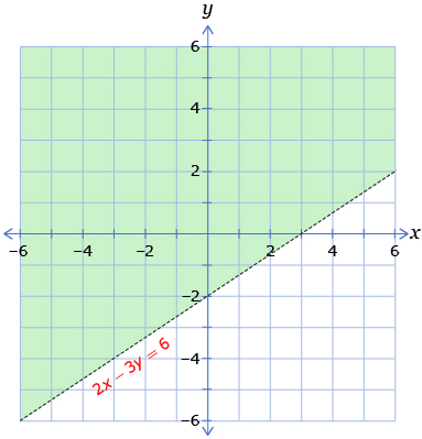
![]() Save your responses in your course folder.
Save your responses in your course folder.
Share 2
With a classmate, compare your strategies for each of the exercises in Try This 4. If both you and your partner used the same strategy, see if you can develop a second strategy together. Discuss the relative benefits and drawbacks of each strategy.
1.9. Explore 5
Module 4: Quadratic Equations and Inequalities
Using a Test Point to Determine the Graph of an Inequality
Watch Using a Test Point to see one way to approach Try This 4, question 2 using a test point. In the video, a misconception is introduced. Pay attention to what the misconception is and how to avoid it.
Self-Check 2

Test your skills by completing Understanding Inequalities.
Working with Constraints
Linear and quadratic inequalities can be used to model situations with constraints. For example, an architect may be constrained by such factors as the available space, the cost of the project, and environmental considerations.

Launch Graphing Linear Inequalities. In the lower right corner of the window, click on the green bar showing the page number. Select page 9, and then complete the exercises on pages 9 to 12. What constraints are imposed in this example situation?
Work through “Example 4” on page 495 in the textbook to see how a situation can be modelled with a quadratic inequality. As you read ask yourself what the significance of the solution region is?
Did You Know?

Khan Academy (CC BY-NC-SA 3.0)
You may have noticed in the textbook reading on page 495 that one of the graphs is created with technology. In Try This 1 you used an applet to graph inequalities in two variables. Did you know that you can also use your graphing calculator? Take a look at Graphing Inequalities with a Graphing Calculator.
Try This 5
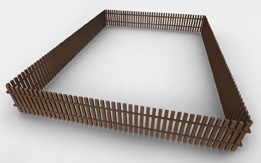
© GP/19600060/Fotolia
A designer is considering different ways to enclose a rectangular area. One of the constraints of the design is that a maximum of only 20 m of fencing is available.
- Write an inequality in terms of length,
 , and width, w, that represents the constraint.
- Graph the inequality from question 1. You can choose to represent either
 or w on the horizontal axis.
- Assume that another constraint on the length of the enclosed area is modelled by the inequality
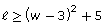 , where
  is the length of the rectangular enclosure and w is the width of the enclosure. Graph the inequality representing the second constraint on the same set of axes you used for the first constraint (question 2).
- Assume that the designer is only interested in whole-number dimensions. List all possible solutions.
![]() Save your answers in your course folder.
Save your answers in your course folder.
Self-Check 3
1.10. Connect
Module 4: Quadratic Equations and Inequalities
Connect
Lesson 7 Assignment
Open the Lesson 7 Assignment you saved in your course folder at the start of this lesson. Complete the assignment.
![]() Save your work in your course folder.
Save your work in your course folder.

Photos.com/Thinkstock
Project Connection

© wong yu liang/29976438/Fotolia
Go to Module 4 Project: Imagineering. Complete Step 5: Operations/Management.
![]() Save your work in your course folder.
Save your work in your course folder.
Going Beyond
Previously in this module you studied systems of linear-quadratic and quadratic-quadratic equations. The solution to such systems can be determined graphically by identifying the point(s) of intersection between the graphs of the equations in the system.
How would you determine the solution to a system of inequalities graphically? In other words, if you graphed two linear or quadratic inequalities on the same coordinate plane, where would your solution points be?
Try This 5 is an example of a system of inequalities. In that exercise you considered multiple constraints of a problem, and you determined possible solutions that satisfied both constraints.
Linear programming is the use of linear inequalities to model the constraints of a problem. The model can then be used to determine possible solutions by analyzing the overlapping shaded areas, known as feasible regions.

Screenshot reprinted with permission of ExploreLearning
Launch Linear Programming - Activity A to graph up to five linear inequalities at once. The program also introduces the concept of an objective function. The objective function is an equation whose value mathematicians try to maximize or minimize by substituting values of the feasible region into it. In a real-world application, this objective function might be profit, cost, area, and so on.
1.11. Lesson 7 Summary
Module 4: Quadratic Equations and Inequalities
Lesson 7 Summary

© Shu He
In this lesson you investigated the following questions:
- How are the properties of linear and quadratic inequalities in two variables related to their graphs?
- How are linear and quadratic inequalities in two variables applied in design?
You explored linear inequalities and quadratic inequalities in two variables, and you learned how to graph these inequalities. To graph a linear or quadratic inequality, you must answer two key questions:
- How do I graph the boundary?
- How do I know which half-plane should be shaded?
The following table summarizes the properties of the graph of linear and quadratic inequalities given each type of inequality symbol.
| < | ≤ | > | ≥ | |
| Boundary Type | dashed | solid | dashed | solid |
| Shading Relative to Boundary when y Is Isolated | below | below | above | above |
| Linear Inequality |  |
 |
 |
 |
| Quadratic Inequality |  |
 |
 |
 |
You also learned how to use the graphs of linear and quadratic inequalities to model problems involving constraints. These models are used in design and other industries to find possible solutions to problems.
In the final lesson of this module you will investigate solutions to quadratic inequalities in one variable. You will investigate both graphical and algebraic methods as solution strategies.