Lesson 2
| Site: | MoodleHUB.ca 🍁 |
| Course: | Math 20-1 SS |
| Book: | Lesson 2 |
| Printed by: | Guest user |
| Date: | Thursday, 4 December 2025, 2:15 AM |
Description
Created by IMSreader
1. Lesson 2
Module 7: Absolute Value and Reciprocal Functions
Lesson 2: Absolute Value Functions
Focus

Jupiterimages/ liquidlibrary/Thinkstock
Artwork often shows reflections of landscapes and portraits. Many graphic designs also exhibit this type of symmetry. In the case of computer-generated art, it can be quite simple to create a design showing reflective symmetry once one-half of the design is created. Software can be used to duplicate the image and align it to create the desired effect. On the other hand, traditional artwork, such as paintings and sketches, do not provide the artist with the “cut-and-paste” option. Rather, the artist must not only create the same scene twice, but must also pay careful attention to the details of the reflected part to ensure accuracy.
In this lesson you will investigate absolute value functions. You will develop techniques to sketch the graphs of absolute value functions based on corresponding linear and quadratic functions. You will discover that you can employ strategies based on reflections in the coordinate plane that will help you to construct the appropriate graphs.
Outcomes
At the end of this lesson you will be able to
- create a table of values for
 , given a table of values for
- generalize a rule for writing absolute value functions in piecewise notation
- sketch the graph of
 ; state the intercepts, domain, and range; and explain the strategy used
Lesson Questions
In this lesson you will investigate the following questions:
- How do the properties of compare to those of
 ?
?
- How can absolute value functions be written in piecewise notation?
Assessment
Your assessment may be based on a combination of the following tasks:
- completion of the Lesson 2 Assignment (Download the Lesson 2 Assignment and save it in your course folder now.)
- course folder submissions from Try This and Share activities
- additions to Module 7 Glossary Terms and Formula Sheet
- work under Project Connection
Materials and Equipment
You will need a graphing calculator and graph paper.
1.1. Launch
Module 7: Absolute Value and Reciprocal Functions
Launch
Do you have the background knowledge and skills you need to complete this lesson successfully? This section, which includes Are You Ready? and Refresher, will help you find out.
Before beginning this lesson you should be able to
- describe a function and use function notation
- graph linear functions
- graph quadratic functions
1.2. Are You Ready?
Module 7: Absolute Value and Reciprocal Functions
Are You Ready?
Complete these questions. If you experience difficulty and need help, visit Refresher or contact your teacher.
- Define function and explain function notation. Answer
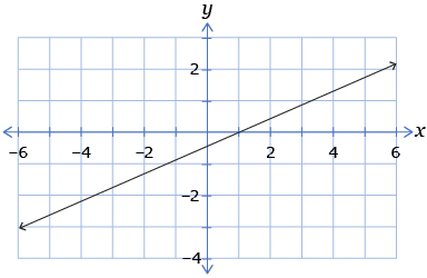
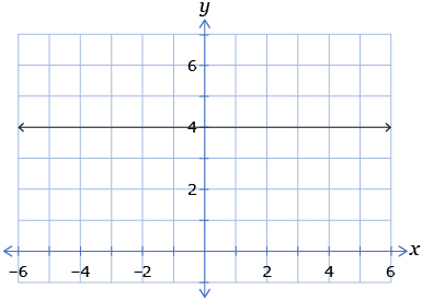
- Graph each linear function on a sheet of graph paper.
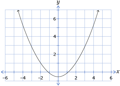
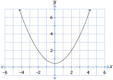
- Graph each quadratic function on a sheet of graph paper.
How did the questions go? If you feel comfortable with the concepts covered in the questions, skip forward to Discover. If you experienced difficulties, use the resources in Refresher to review these important concepts before continuing through the lesson.
1.3. Refresher
Module 7: Absolute Value and Reciprocal Functions
Refresher
Use “Introduction to Functions” to work with expressions written in function notation. Watch the video to review what a function is and to see how functions are written using function notations.

Khan Academy - CC BY-NC-SA 3.0
Open “Linear Function Graphs.” Watch the video to review how to graph a linear function using a table of values.
Khan Academy - CC BY-NC-SA 3.0
Use “Quadratic Functions 1” to review how to graph a linear function using a table of values.

Khan Academy - CC BY-NC-SA 3.0
Go back to the Are You Ready? section, and try the questions again. If you are still having difficulty, contact your teacher.
1.4. Discover
Module 7: Absolute Value and Reciprocal Functions
Discover

In this Discover section you will engage in guided exploration of the graphs of absolute value functions. Using applets, you will manipulate the parameters of both linear and quadratic functions to observe what happens when you take the absolute value of those graphs.
At the end of this section, see if you can relate your discoveries to the cartoon strip.
Try This 1
Part A: The Absolute Value of a Linear Function
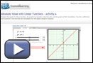
Screenshot reprinted with permission of ExploreLearning
Step 1: Launch the Absolute Value with Linear Functions – Activity A applet. A window will open that shows the graph of a linear function in the right panel. In the left panel, you can manipulate the equation of the graph. Focus only on the top half of the activity, leaving the assessment questions for later.
Step 2: Change the graph to y = 0.5x − 1. Notice that the graph adjusts to the changes in the equation.
Step 3: In the left panel, select “Show ![]() .” The blue graph that appears is the graph of the absolute value of the linear function.
.” The blue graph that appears is the graph of the absolute value of the linear function.
Step 4: In the left panel, select “Show probe.” This function displays a vertical line on the graph and a table comparing the y-coordinates of the functions displayed on the graph.
Click and drag the “probe line” to different x-coordinates across the grid. Compare the y-values of the linear function and absolute value function. When are they identical? When are they different?
Step 5: Leave the “Show y = ax + b” and “Show ![]() ” selections on. Drag the b-slider to see how the graph is affected. Then do the same with the a-slider.
” selections on. Drag the b-slider to see how the graph is affected. Then do the same with the a-slider.
Part B: The Absolute Value of a Quadratic Function
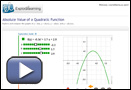
Screenshot reprinted with permission of ExploreLearning
Step 1: Launch the Absolute Value of a Quadratic Function applet. A window will open that shows the graph of a linear function in the right panel. In the left panel, you can manipulate the equation of the graph. Focus only on the top half of the activity, leaving the assessment questions for later.
Step 2: Change the graph to y = 0.7x2 + −5.0x + 2.6. Notice that the graph adjusts to the changes in the equation.
Step 3: In the left panel, select “Show y = |f(x)|.” The black graph that appears is the graph of the absolute value of the quadratic function. Deselect “y = f(x)” to see the graph in its entirety. Then select it again before proceeding to the next step.
Step 4: With both “y = f(x)” and “![]() ” selected, drag the b-slider in the left panel to see how the graph is affected. Then repeat Step 4 with only the "
” selected, drag the b-slider in the left panel to see how the graph is affected. Then repeat Step 4 with only the "![]() ” selected.
” selected.
Step 5: Adjust the a-slider so that a < 0. Repeat Step 4 to see what happens when the a-parameter is negative.
Analysis
Complete the following analysis questions based on your observations from Part A and Part B.
- What is the shape of the absolute value of a linear function?
- What is the shape of the absolute value of a quadratic function?
- In what part of the coordinate plane will you find the graph of an absolute value function? Why?
- How does the graph of the absolute value of a linear or a quadratic function compare with the graph of the corresponding linear or quadratic function?
- How would you instruct someone to graph the absolute value of a linear or quadratic function without the aid of technology?
![]() Save your work in your course folder. You will confirm these results later in the lesson.
Save your work in your course folder. You will confirm these results later in the lesson.
1.5. Explore
Module 7: Absolute Value and Reciprocal Functions
Explore
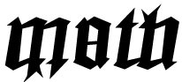
Can you read the words in the graphic shown? Now try reading it upside down. (You may need to print the page first.) An ambigram is a word graphic that can be read from more than one perspective. In the image, you may have noticed that the word “math” is the same when read upside down! Ambigrams are commonly used in the tattooing industry for this special property. Indeed, a design that can be read by both the onlooker as well as the tattooed person has a practical appeal.
In this lesson you will discover how the graphs of absolute value functions are similar to ambigrams. Besides exploring their graphs, you will also consider an alternate way of expressing absolute value functions using a special type of notation.
Here are some of the words you will want to define in Module 7 Glossary Terms in this lesson:
- critical point
- piecewise notation
1.6. Explore 2
Module 7: Absolute Value and Reciprocal Functions
Absolute value functions have the form ![]() , where f(x) is a function.
, where f(x) is a function.
Retrieve the results from the Discover section. In that activity you discovered that the graphs of absolute value functions are found either on or above the x-axis. In Try This 2 you will use tables to find out why.
Try This 2
Consider the functions f(x) = x − 2 and ![]() .
.
- Determine the y-coordinates for each of the given x-coordinates in each function. Record your answers in a table like the one that follows.
Table 1: Table of Values for y = f(x) and y = g(x) x y = f(x) y = g(x) −6 −3 0 3 6
- Plot the ordered pairs for each function on the same graph paper.
![]() Save your work in your course folder. Save Table 1 for future reference.
Save your work in your course folder. Save Table 1 for future reference.
Share 1
With a classmate, discuss the following questions based on Try This 2.
- Compare your answers in the second and third columns of Table 1. When are the values the same? When are they different?
- Based on Table 1 and the graph, explain why the graph of the absolute value function y = g(x) is not found below the x-axis.
- Assume that a student chose different x-values for Table 1 (as shown in the following table) to use for sketching the graph of y = g(x).
x y = f(x) y = g(x) 2 3 4 5 6
- How could this selection of x-values lead the student to an incorrect graph?
- How do you choose values of x so that you do not sketch an incorrect graph?
- How could this selection of x-values lead the student to an incorrect graph?
![]() Save your responses in your course folder.
Save your responses in your course folder.
1.7. Explore 3
Module 7: Absolute Value and Reciprocal Functions
In Try This 2 you learned how to use a table to graph an absolute value function ![]() .
.
You can also use the graph of a function to graph the absolute value of that function. Launch the Graphing Absolute Value Functions: Reflection Method piece to see how.
From the multimedia piece, you learned that you can graph the absolute value of a function by working with the graph of the original function.
In fact, the graph of the absolute value of a function is the same as the graph of the original function, except that any part of the graph that is below the x-axis is reflected across the x-axis.
Turn to part b) of “Example 2” on pages 372–373 in your textbook. This example shows how the absolute value function of the form f(x) = ax2 + bx + c is graphed. As you work through the example, look for the answers to the following questions:
- Was the table method or the reflection method used?
- Why is it necessary to complete the square on the quadratic function?
Self-Check 1
Take a moment to check your understanding of the concepts presented so far. The questions are not for marks, but for you to assess your own learning. Have some scrap paper handy to work through the problems. You may wish to save your rough work in your course folder for future reference. If you make a mistake, don’t worry. You can reset the question, and then try again.
- Complete the table for the functions y = f(x) and
 . Answer
x y = f(x) y = |f(x)|
−3 7 −2 5 0 1 2 −3 5 −9
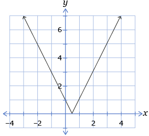
- Which of the following graphs is the graph of
 from question 1?
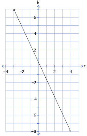 B.
B. 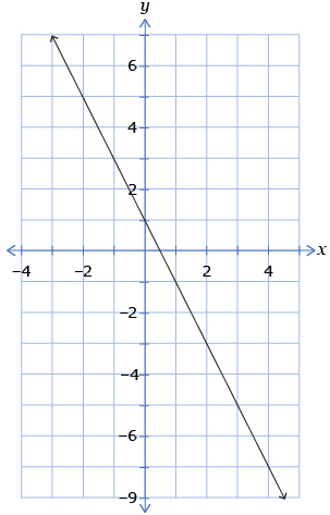
- D.
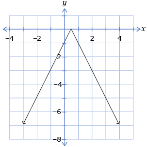
- The point (−1, −2) is on the graph of y = f(x). Which of the following is the corresponding point on the graph of
 ?
?
- (−1, −2)
- (1, −2)
- (−1, 2)
- (1, 2)
- Which graph(s) below will not change if you graph the absolute value of the corresponding function?
1.8. Explore 4
Module 7: Absolute Value and Reciprocal Functions
In the next section of the lesson you will study the properties of the graphs of absolute value functions. You will compare these properties to those of linear functions and quadratic functions.
Try This 3
Part A: Properties of the Absolute Value of a Linear Function
- Retrieve your graph from Try This 2.
- Identify the properties listed in Table 2 for each function. Complete the table.
Table 2: Properties of y = f(x) and y = g(x) y = f(x) y = g(x) Domain Range x-intercept y-intercept
- Compare and contrast the properties of y = f(x) and y = g(x).
Part B: Properties of the Absolute Value of a Quadratic Function
- Identify the properties listed for each of the quadratic functions in Table 3.
Table 3: Properties of Quadratic Functions y = x2 y = x2 − 4 y = x2 + 4 Domain Range x-intercept y-intercept
- Identify the properties listed for the absolute value of each function listed in Table 4.
Table 4: Properties of the Absolute Value of Quadratic Functions y = |x2| y = |x2 − 4| y = |x2 + 4| Domain Range x-intercept y-intercept
- Compare and contrast the properties of the functions in Table 3 and the corresponding absolute value functions in Table 4.
- Graph the following pairs of graphs.
- Based on your observations, when is the graph of y = f(x) identical to the graph of
 ?
?
![]() Save your answers in your course folder.
Save your answers in your course folder.
Share 2
With a classmate, compare your responses to Try This 3. Answer the following questions.
- How do the properties of y = f(x) compare to those of
 ?
?
- What other properties of absolute value functions can you identify?
Make any necessary revisions to your own work based on the discussion. Save your work in your course folder.
1.9. Explore 5
Module 7: Absolute Value and Reciprocal Functions
Self-Check 2
Turn to page 376 of your textbook to practise applying the concepts that you have learned. Complete questions 5.b., 6.e., 7.a., and 8.c. Check the solutions in the back of the textbook to make sure you are doing the questions correctly. You may also want to review relevant parts of the lesson as you work through the questions.
A critical point on the graph of an absolute function is a point where the graph changes direction. Critical points on the graph of an absolute value function are found on the x-axis. In the next part of the lesson you will learn how to express absolute value functions based on the location of their critical points.
Try This 4
Retrieve your graph from Try This 2. It should look like the following graph.
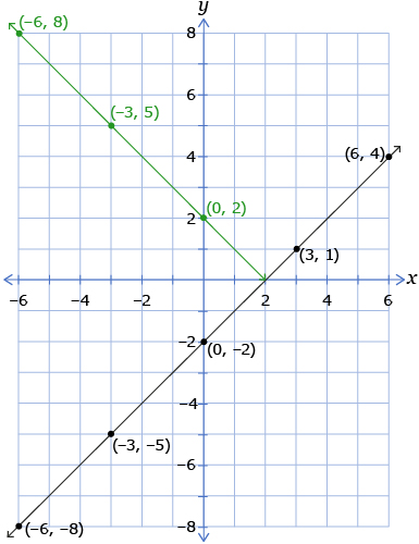
- Where is the critical point?
- For all x-values greater than the critical point, what is the expression for obtaining the corresponding y-value?
- For all x-values less than the critical point, what is the expression for obtaining the corresponding y-value?
![]() Save your answers in your course folder.
Save your answers in your course folder.
1.10. Explore 6
Module 7: Absolute Value and Reciprocal Functions
In your graph from Try This 4, the single critical point is found at x = 2. It is at this point that the graph of ![]() changes direction. Notice that for all values of x greater than 2, the corresponding y-values on the graph are equal to x − 2. However, for all values of x less than 2, the corresponding y-values are equal to −(x − 2).
changes direction. Notice that for all values of x greater than 2, the corresponding y-values on the graph are equal to x − 2. However, for all values of x less than 2, the corresponding y-values are equal to −(x − 2).
This leads to a new notation known as piecewise notation. You can use this notation to express ![]() as
as
![]()
It is called piecewise notation because it breaks the function into distinct “pieces.” Theoretically, you could break the function into as many pieces as you want. However, the generally accepted practice is to break the function into pieces at the critical points.
Turn to part d) of “Example 1” on pages 370–372 of your textbook to see how you can express in piecewise notation. As you read, focus on finding the answers to these questions:
- How was the value
 obtained?
 - How does the negative in the expression −(2x − 3) affect the y-values when
 ?
?
Try This 5
Consider the function ![]() . Express the function using piecewise notation. (Access the hints if you need help.)
. Express the function using piecewise notation. (Access the hints if you need help.)
- What do I do first?

- How do I find critical points?
- How do I use critical points?
Compare your final answer with the one in the textbook. You can find it on page 374, part d).
Self-Check 3
Turn to page 377 of your textbook to practise applying the concepts that you have learned. Complete questions 9.a. and b., 10.a. and c., 12, and 14. Check the solutions in the back of the textbook to make sure you are doing the questions correctly. You may also want to review relevant parts of the lesson as you work through the questions.
1.11. Connect
Module 7: Absolute Value and Reciprocal Functions

Open your copy of Lesson 2 Assignment, which you saved in your course folder at the beginning of this lesson. Complete the assignment.
![]() Save all your work in your course folder.
Save all your work in your course folder.
Project Connection
In this lesson you analyzed absolute value functions and their graphs. You are now ready to move on to the next phase of your project. Go to your project now and complete Step 2.
![]() Save all your work in your course folder.
Save all your work in your course folder.
Going Beyond
You learned in this lesson that you can construct the graph of the absolute value of a function by reflecting all parts of the graph of the function across the x-axis.
The principle of reflection is also applicable in art, whether it is found in a watercolour painting or a graphic design.
In this Going Beyond, you are challenged to create your own ambigram. You may want to try your name or a word. Do an Internet search using the keywords “ambigram examples.” From what other views can you view your ambigram? Get inspired!
Stuck as to how to make a “w” look like a “q”? You can also search the Internet for an “ambigram generator.” Input your expression or name and let the generator work the magic!
![]() Save your work in your course folder.
Save your work in your course folder.
1.12. Lesson 2 Summary
Module 7: Absolute Value and Reciprocal Functions
Lesson 2 Summary

© MENZAGO/7241364/Fotolia
In this lesson you investigated the following questions:
- How do the properties of y = f(x) compare to those of
 ?
?
- How can absolute value functions be written in piecewise notation?
Absolute value functions have the form ![]() , where f(x) is a function.
, where f(x) is a function.
In this lesson you learned how to graph absolute value functions. You discovered that you can do this by converting the y-values of all points located underneath the x-axis into positive values. The effect of doing this is to reflect all parts of the graph underneath the line y = 0 across the x-axis.
You also compared the properties of y = f(x) to those of ![]() . You found that the domain is the same for both functions, but that the range of the absolute value function depends on the range of the original function. Generally, the range of
. You found that the domain is the same for both functions, but that the range of the absolute value function depends on the range of the original function. Generally, the range of ![]() is
is ![]() .
.
Piecewise notation is a special way of expressing an absolute value function by describing each part of the function based on divisions at the critical points. You learned that, in general, ![]() .
.
In the next lesson you will investigate absolute value equations. You will learn how to determine the solutions of such equations both graphically and algebraically.