Lesson 1
| Site: | MoodleHUB.ca 🍁 |
| Course: | Math 30-1 SS |
| Book: | Lesson 1 |
| Printed by: | Guest user |
| Date: | Tuesday, 9 December 2025, 10:35 PM |
Description
Created by IMSreader
1. Lesson 1
Module 3: Polynomial Functions
Lesson 1: Sketching Polynomial Functions
Focus

adapted from Photodisc/Thinkstock
The spaces, shapes, and forms of graphic design rely on many principles of mathematics. M.C. Escher, one of the world’s most famous graphic artists, is noted for the complex mathematical aspects of his work. Today, graphic design is a competitive industry that is dependant on computers and design software. Designers are expected to grasp fundamental math principles and concepts to solve design problems.
A graphic artist may want to capture the contour of an abstract design. A curve following the graph of a polynomial function may be useful in the design. A polynomial function that could be used to describe this curve is f(x) = 23x4 − 69x3 − 2208x2 + 8924x + 11 040. This same function can be written in an equivalent factored form, f(x) = 23(x + 10)(x + 1)(x − 6)(x − 8). Both forms express the same polynomial, but each form will allow you to more easily obtain different information.
In this lesson you will learn how the factored form and the expanded form of a function can help identify different behaviours and characteristics about the corresponding graph.
Lesson Outcomes
At the end of this lesson you will be able to sketch the graph of a polynomial function given the equivalent expanded and factored forms, without the use of technology.
Lesson Questions
You will investigate the following questions:
- How does the expanded form of a polynomial function help identify the end behaviour of the corresponding graph?
- How does the factored form of a polynomial function help identify the x-intercepts of the corresponding graph?
Assessment
Your assessment may be based on a combination of the following tasks:
- completion of the Lesson 1 Assignment (Download the Lesson 1 Assignment and save it in your course folder now.)
- course folder submissions from Try This and Share activities
- additions to Glossary Terms
- work under Project Connection
Self-Check activities are for your own use. You can compare your answers to suggested answers to see if you are on track. If you are having difficulty with concepts or calculations, contact your teacher.
Remember that the questions and activities you will encounter provide you with the practice and feedback you need to successfully complete this course. You should complete all questions and place your responses in your course folder. Your teacher may wish to view your work to check on your progress and to see if you need help.
Time
Each lesson in Mathematics 30-1 Learn EveryWare is designed to be completed in approximately two hours. You may find that you require more or less time to complete individual lessons. It is important that you progress at your own pace, based on your individual learning requirements.
This time estimation does not include time required to complete Going Beyond activities or the Module Project.
1.1. Launch
Module 3: Polynomial Functions
Launch
Do you have the background knowledge and skills you need to complete this lesson successfully? Launch will help you find out.
Before beginning this lesson you should be able to factor quadratic polynomials of the form x2 + bx + c and ax2 + bx + c.
1.2. Are You Ready?
Module 3: Polynomial Functions
Are You Ready?
Complete the following questions. If you experience difficulty and need help, visit Refresher or contact your teacher.
Completely factor each expression.
If you answered the Are You Ready? questions without difficulty, move to Discover.
If you found the Are You Ready? questions difficult, complete Refresher.
1.3. Refresher
Module 3: Polynomial Functions
Refresher
Source: Khan Academy
(![]() BY-NC-SA 3.0)
BY-NC-SA 3.0)
Watch “Factoring trinomials with a leading 1 coefficient.”
Source: Khan Academy
(![]() BY-NC-SA 3.0)
BY-NC-SA 3.0)
Watch “Factoring trinomials with a non-1 leading coefficient by grouping.”
1.4. Discover
Module 3: Polynomial Functions
Discover
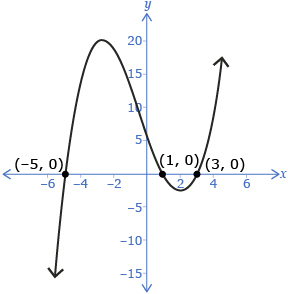
When sketching polynomial functions, one of the characteristics of interest is the behaviour of f(x) (the y-coordinates) as x approaches infinity or negative infinity. This is called end behaviour. Consider the following graph:
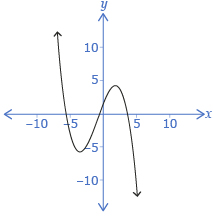
As x approaches −∞, the y-coordinates approach ∞. As x approaches ∞, the y-coordinates approach −∞. Another way to describe this is to think of the graph as “starting” in negative x-values and “ending” in positive x-values. So, you would say that this graph starts in quadrant 2 and ends in quadrant 4.
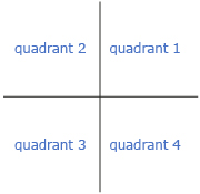
Recall how quadrants on the Cartesian plane are numbered.
Try This 1
Step 1: Use End Behaviour Explorer to look for patterns in end behaviour. When the applet starts, a first-degree (linear) function is shown. Change the a and b sliders, paying attention to how the end behaviour of the function changes.
The degree of a polynomial is equal to the highest exponent of the variable.
Step 2: Repeat for functions of degree 2, 3, 4, and 5.
Step 3: You may choose to create a chart to record and organize your observations.
- Which slider(s) affects the end behaviour of the graphs?

- Describe how the degree of the polynomial and the slider(s) identified in question 1 affects the end behaviour of the graphs.
![]() Save your responses in your course folder.
Save your responses in your course folder.
Share 1
With a partner or in a group, discuss and summarize in a paragraph how the different parts of the polynomial can be used to predict end behaviour.
![]() If required, save a record of your discussion in your course folder.
If required, save a record of your discussion in your course folder.
1.5. Explore
Module 3: Polynomial Functions
Explore
All of the functions that were graphed in Try This 1 are called polynomial functions. A polynomial function is any function that can be written as the sum or difference of terms where the variables have only positive integer exponents.
The formal definition for a polynomial function is any function that can be written in the following form: f(x) = anxn + an − 1xn − 1 + an − 2xn − 2 + … + a2x2 + a1x + a0, where
- n is a whole number
- x is a variable
- the coefficients a0, a1, a2, …, an are real numbers1
The following are all examples of polynomial functions:
- y = 3x + 1
- k(x) = (2x − 1)(x + 3)
Although the last function, k(x), doesn’t look like it fits the definition, the key is that it can be written in the form shown above. Expanding k(x) results in
The last line is in the form described above; thus, k(x) fits the definition of a polynomial function.
Note that k(x) was originally written in factored form. It has two factors: 2x − 1 and x + 3.
For more examples of how to identify polynomial functions, read “Example 1” on page 108 of the textbook.
Self-Check 1
Complete Identify the Polynomial Functions.
1 Source: Pre-Calculus 12. Whitby, ON: McGraw-Hill Ryerson, 2011. Reproduced with permission.
1.6. Explore 2
Module 3: Polynomial Functions
When a polynomial is written in expanded form and in order of decreasing exponents, the first term is called the leading term. The first term’s coefficient is called the leading coefficient.
What you probably discovered in Try This 1 is that when graphing a polynomial function written in expanded form, the end behaviour is completely determined by the degree of the polynomial and the sign of the leading coefficient.
- When the degree of the polynomial is odd, the graph will begin and end in quadrants on different sides of the x-axis.
- When the degree of the polynomial is even, the graph will begin and end in quadrants on the same side of the x-axis.
- The sign of the leading coefficient determines where the graph will begin.
As you read through the examples in the table, pay special attention to how the sign of the leading coefficient determines where the graph begins.
| Polynomial Degree | Sign of Leading Coefficient | End Behaviour | Example | |
| Starting Quadrant | Ending Quadrant | |||
| odd | positive | 3 | 1 |
|
| odd | negative | 2 | 4 |
|
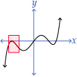
| even | positive | 2 | 1 | 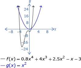 |
| even | negative | 3 | 4 | 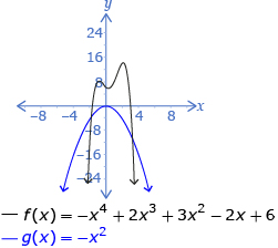 |
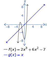
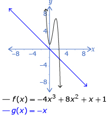
The end behaviour of all odd-degree polynomial functions is the same as y = x or y = −x. Since the graphs of y = x and y = −x are easy to remember, so is the end behaviour of all odd functions.
The end behaviour of all even-degree polynomial functions is the same as y = x2 or y = −x2. Since the graphs of y = x2 and y = −x2 are easy to remember, so is the end behaviour of all even functions.
You may want to use End Behaviour Explorer again to confirm these patterns.
Self-Check 2
Use your knowledge of polynomial function end behaviour to answer the following questions. You should be able to answer all of the questions without actually graphing the functions.
- Use the degree and the sign of the leading coefficient of each function to describe the end behaviour of the corresponding functions. State the value of the y-intercept.2
- Use the degree and the sign of the leading coefficient of each function to describe the end behaviour of the corresponding functions. State the value of the y-intercept.
2 Source: Pre-Calculus 12. Whitby, ON: McGraw-Hill Ryerson, 2011. Reproduced with permission.
1.7. Explore 3
Module 3: Polynomial Functions
Try This 2

Use Factored Form Explorer to look for relationships between the parameters (a, b, c, d, and e) and the x-intercepts in the graphs. When the applet starts, a first-degree function is shown. Change the a and b sliders, paying attention to how the graph changes. You may want to click the Show x-intercepts box to see more information.
Repeat for functions of degree 2, 3, 4, and 5. You may want to use a table like the one shown to organize your results.
| Degree | Type of Function | Observations |
| 1 | linear | |
| 2 | quadratic | |
| 3 | cubic | |
| 4 | quartic | |
| 5 | quintic |
![]() Save your responses in your course folder.
Save your responses in your course folder.
Share 2
With a partner or in a group, share your observations from Try This 2. As part of your discussion, consider the following questions:
- How do the parameters in the functions (a, b, c, d, e, and f) relate to the x-intercepts of the corresponding graph?
- Is there an algebraic reason for your observation in question 1?
![]() If required, save a summary of your discussion in your course folder.
If required, save a summary of your discussion in your course folder.
1.8. Explore 4
Module 3: Polynomial Functions
In Try This 2 you probably discovered that x-intercepts are directly related to the factors of a polynomial function. The following example illustrates the relationship between a polynomial function and the x-intercepts of its graph.
What are the x-intercepts of the graph of f(x) = 0.4(x − 3)(x + 5)(x − 1)?
You need two key pieces of information:
- All x-intercepts have y-coordinates of zero.
- The zero-product property: If s and t are real numbers and st = 0, then either s must be zero, t must be zero, or they are both zero. (This can be extended to the product of any number of numbers.)
The zero-product property may sound confusing, but it’s just a formal way of stating what you already know: if you multiply some numbers together, the only way to get zero is if one (or both) of those numbers is zero. Here are some examples:
- 5 × 0 = 0
- 0 × 17x − 3 = 0

Since the x-intercepts have y-coordinates of zero, you are looking for values that make the following equation true:
0.4(x − 3)(x + 5)(x − 1) = 0
The left side is the product of four real numbers: 0.4, x − 3, x + 5, and x − 1. The only way a product of numbers can be zero is if one (or more) of those numbers is zero (the zero-product property). Thus,
0.4 = 0 (1)
x − 3 = 0 (2)
x + 5 = 0 (3)
x − 1 = 0 (4)
Equation (1) is false, so it can be ignored. Solving the other three equations gives three values of x that make the original equation true:
x = 3
x = −5
x = 1
These make the polynomial function zero, so they are the x-intercepts. Graphing the polynomial function confirms this.
Self-Check 3
State the x-intercepts of the graphs of the following functions without graphing them.
1.9. Explore 5
Module 3: Polynomial Functions
Try This 3
Open Factored Form Explorer again. Choose a polynomial of degree 5. Set the a slider to 0.5. Manipulate the values for b, c, d, e, and f to see what happens when two or more factors are the same. You may want to look at the number of x-intercepts and what happens in the vicinity of each x-intercept.
- Record your observations in a table similar to the one shown.
Number of Factors that Are the Same Number of x-intercepts Sketch or Screen Capture of the Graph at the x-intercept of the Corresponding Repeated Factor Does the graph cross the x-axis at the x-intercept corresponding to the repeated factor? 0 5 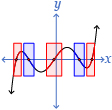
yes 2 
3 4 5 - Summarize the relationship between the number of repeating factors and the behaviour of the graph at the corresponding x-intercept.
![]() Save your responses in your course folder.
Save your responses in your course folder.
The shape would look similar to this, but the x-intercepts will vary.
 |
or | 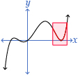 |
1.10. Explore 6
Module 3: Polynomial Functions
In Try This 3 you may have discovered that the number of times a factor is duplicated affects the graph’s behaviour around the corresponding x-intercept.
- If a factor is repeated an odd number of times, the function changes sign (the graph crosses the x-axis) at the corresponding x-intercept.
- If a factor is repeated an even number of times, the function does not change sign (the graph touches but does not cross the x-axis) at the corresponding x-intercept.
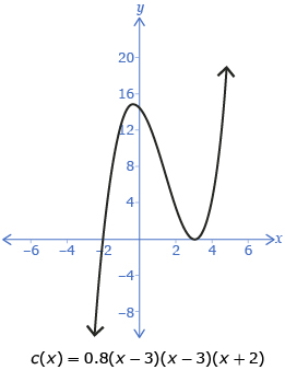
Consider the function c(x) = 0.8(x − 3)(x − 3)(x + 2). The factor x + 2 is repeated an odd number of times, so the function changes sign at the corresponding x-intercept (x = −2). The factor x − 3 is repeated an even number of times, so the function does not change signs at the corresponding x-intercept (x = 3).
Mathematicians would say that the factor x − 3 has a multiplicity of 2 and that the factor x + 2 has a multiplicity of 1.
Read “Example 1” on pages 138 and 139 of the textbook for two more examples concerning multiplicity of factors and x-intercepts. Pay particular attention to
- “multiplicity (of a zero)” in the left column (Notice how the graph “flattens” near an x-intercept of multiplicity 3.)
- the analysis of the least possible degree of the polynomial
1.11. Explore 7
Module 3: Polynomial Functions
You now have enough information to sketch polynomial functions without the use of technology.
Here is an outline of the steps to use:
Step 1: Determine the end behaviour by looking at the degree of the polynomial and the sign of the leading coefficient.
Step 2: Factor the polynomial if it is not given in the problem.
Step 3: Determine the x-intercepts by looking at the factors of the polynomial.
Step 4: Determine the y-intercept by substituting zero into the function.
Step 5: Determine the nature of the x-intercepts (whether there is a sign change) by looking at the multiplicity of the polynomial’s factors.
Step 6: Draw a smooth curve through the x- and y-intercepts.
Watch Sketching Polynomial Functions to see an example of graphing a function without using technology.
Self-Check 4
- For each of the following functions, factor the function and create a sketch without technology.
- For each of the following functions, create a sketch without technology.
![]()
- Complete question 3 on page 114 in the textbook. Answer
Add the following terms to your copy of Glossary Terms:
- degree (of a polynomial)
- end behaviour
- leading coefficient
- multiplicity (of a factor)
- polynomial function
- zero-product property
1.12. Connect
Module 3: Polynomial Functions
Complete the Lesson 1 Assignment that you saved in your course folder at the beginning of the lesson. Show work to support your answers.
![]() Save your responses in your course folder.
Save your responses in your course folder.
Project Connection
Go to Module 3 Project: Graphic Design Using Polynomials, and read over all project requirements to become familiar with what you will be doing and how you will be assessed.
Complete Part 1 of the Module 3 Project.
![]() Save your responses in your course folder.
Save your responses in your course folder.
Going Beyond
It should be noted that the end behaviour described in this lesson was generalized by looking at the graphs of many functions. This is not a mathematical proof. In later courses you will learn formal methods for proving these conclusions.
The following shows an informal proof of the end behaviour for f(x) = 2x4 + 3x3 − x2 + 5x.
Factoring out 2x4 results in the following equivalent function:
Now, think about what happens as x gets larger and larger:
As x gets larger, the fractions become smaller and smaller. A mathematician would say that as x approaches infinity, the fractions approach zero. So, as x approaches infinity, you can informally write
And this is exactly the end behaviour expected for an even function: as x approaches ∞, y also approaches ∞.
Similar reasoning can be used to show that as x approaches −∞, y approaches positive ∞—again, the end behaviour you expect for an even-degree function.
1.13. Lesson 1 Summary
Module 3: Polynomial Functions
Lesson 1 Summary
In this lesson you learned how to sketch the graphs of polynomial functions. You learned that
- end behaviour can be determined by the degree and sign of the leading coefficient
- x-intercepts can be determined by looking at the factors of the polynomial
- the graph behaviour at the x-intercepts can be determined by examining the multiplicity of the corresponding factors of the polynomial
- the y-intercept can be determined by substituting zero for x
All functions of degree 3 or higher were shown in both expanded and factored forms. You will learn how to factor these in the next lesson.