Lesson 3
| Site: | MoodleHUB.ca 🍁 |
| Course: | Math 30-1 SS |
| Book: | Lesson 3 |
| Printed by: | Guest user |
| Date: | Tuesday, 9 December 2025, 11:17 PM |
Description
Created by IMSreader
1. Lesson 3
Module 2: Radical Functions
Lesson 3: Solving Radical Equations Graphically
Focus
Objects that are moving with accelerated motion can be described using radical equations. It is common to find objects with an accelerated motion used in many sports. One such sport is lacrosse, Canada’s official summer sport.

Photodisc/Thinkstock
Lacrosse originated in North America, and there are now professional and amateur leagues across Canada. Today, lacrosse is played both indoors and outdoors by men’s and women’s teams.
In lacrosse, a stick with a net at one end is used to throw a hard rubber ball. You can use radical equations to determine the velocity, distance, or acceleration of the ball when thrown.
Previously in this module, you graphed radical functions. How can graphs of radical functions be used to help determine the solution to radical equations?
Lesson Outcome
At the end of this lesson you will be able to determine graphically an approximate solution to a radical equation.
Lesson Question
In this lesson you will investigate the following question:
- How can you determine the solution to a radical equation using graphs?
Assessment
Your assessment may be based on a combination of the following tasks:
- completion of the Lesson 3 Assignment (Download the Lesson 3 Assignment and save it in your course folder now.)
- course folder submissions from Try This and Share activities
- additions to Glossary Terms and Formula Sheet
- work under Project Connection
1.1. Launch
Module 2: Radical Functions
Launch
Do you have the background knowledge and skills you need to complete this lesson successfully? Launch will help you find out.
Before beginning this lesson, you should be able to solve radical equations using algebra.
1.2. Are You Ready?
Module 2: Radical Functions
Are You Ready?
Complete these questions. If you experience difficulty and need help, visit Refresher or contact your teacher.
- Solve the following equations algebraically.
- What are extraneous roots, and why do they occur? Answer
- Graphically solve the equation 2x2 − 4x = 6. Answer
If you answered the Are You Ready? questions without difficulty, move to Discover.
If you found the Are You Ready? questions difficult, complete Refresher.
1.3. Refresher
Module 2: Radical Functions
Refresher

Khan Academy
(c BY-NC-SA 3.0)
Go to “Solving Radical Equations” to review how to solve radical equations.

Review how to solve radical equations by working through Solving a Radical Equation. Depending on your browser, you may need to choose Radical Equations from the menu. From the five icons at the top of the page, choose Tutorial (the middle icon) and then choose Solving a Radical Equation.

Khan Academy
(c BY-NC-SA 3.0)
The video “Extraneous Solutions to Radical Equations” demonstrates how to determine if a solution is extraneous.

Review how to solve quadratic equations graphically by working through Solving a Quadratic Equation by Graphing. Depending on your browser, you may need to choose Solving Quadratic Equations: Using Graphs from the menu. From the five icons at the top of the page, choose Tutorial (shaped like a blackboard) and work through Solving a Quadratic Equation by Graphing.
The video Solving a Quadratic Equation by Graphing a Related System of Equations is a review of solving quadratic equations graphically.
Go back to the Are You Ready? section and try the questions again. If you are still having difficulty, contact your teacher.
1.4. Discover
Module 2: Radical Functions
Discover
Try This 1
- Graph the function

- Use this graph to solve the radical equation
 Describe the process or strategy that you used.
 - Could there be other methods to solve this equation? If yes, describe the process.
- Solve the equation
 algebraically.
![]() Save your responses in your course folder.
Save your responses in your course folder.
Share 1
With a partner or group, discuss the following questions based on the graph you created in Try This 1.
- Do you prefer an algebraic or a graphical method for solving a radical equation? Explain why.
- Are there advantages or disadvantages of the graphical method compared to the algebraic method?
![]() If required, place a summary of your discussion in your course folder.
If required, place a summary of your discussion in your course folder.
1.5. Explore
Module 2: Radical Functions
Explore
In Try This 1 you looked at using a graph to solve a radical equation. You will explore two graphical methods used to determine solutions to radical equations.
In Try This 2 you will look at a radical equation that equals zero. How are the roots of a radical equation and the x-intercepts of the graph of the corresponding radical function related?
Try This 2
- Determine the root of
 algebraically.
- Open Relating Roots and x-intercepts.
Slide the blue point on the function to answer the following questions.
- What is the x-intercept of the graph?
- What is the root to the equation
 ?
? - Why is the value you determined in part b the root of the equation?
- What do you notice about your answers to questions 1 and 2? Why do you think this is?
- Do you think this same relationship exists for other radical functions and equations? Why or why not?
![]() Save your responses in your course folder.
Save your responses in your course folder.
Share 2
With a partner or in a group, describe the relationship between the roots of the equation and the x-intercepts of the corresponding graph and explain why you think this is.
![]() If required, place a summary of your discussion in your course folder.
If required, place a summary of your discussion in your course folder.
1.6. Explore 2
Module 2: Radical Functions
In Try This 2 you graphed the function ![]() and determined the x-intercept and root of the equation
and determined the x-intercept and root of the equation ![]() . You should have found that x = 8 is the x-intercept of the graph because the value of the function is 0 when x = 8. This means the roots to a radical equation are equal to the x-intercepts of the graph of the corresponding radical function.
. You should have found that x = 8 is the x-intercept of the graph because the value of the function is 0 when x = 8. This means the roots to a radical equation are equal to the x-intercepts of the graph of the corresponding radical function.
Self-Check 1
Complete “Your Turn” at the end of “Example 1” on page 91 of the textbook. Answers
In Try This 3 a different graphical method will be used to solve a radical equation. Then the solution will be compared to the algebraic method of solving the radical equation.
Try This 3
- Solve the equation
 graphically. Graph each side of the equation as a separate function.
- Determine the x-value at the point(s) where y1 = y2. Make sure to round your answer to the nearest hundredth.
- Following is the algebraic solution. What are the similarities and differences between the solutions to the graphical method and the algebraic method?
Check for extraneous roots. Substitute and
and  into the original equation.
LS RS 
x

LS RS 
x

LS ≠ RS LS = RS
The solution is , or x ≈ 1.73.
![]() Save your responses in your course folder.
Save your responses in your course folder.

1.7. Explore 3
Module 2: Radical Functions
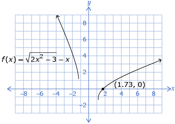
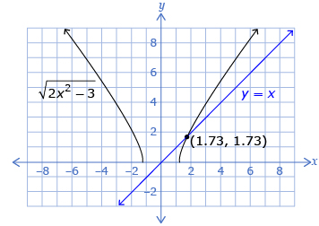
In Try This 3 you may have produced a graph like this.
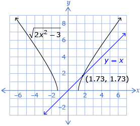
The solution is the x-value at the intersection point of the two graphed functions. Graphically, there is only one solution, approximately 1.73. Algebraically, there were two solutions, ![]() , with one solution being an extraneous root,
, with one solution being an extraneous root, ![]() .
.
In Try This 3 you may have reached the following conclusions:
- The graphical solution is the same as the algebraic solution.
- The algebraic solutions can be given as exact values or approximate values.
- The graphical solutions are given as approximate values.
- The algebraic solutions may have extraneous solutions. The graphical solutions are never extraneous solutions.
Self-Check 2
![]()
1.8. Explore 4
Module 2: Radical Functions
There are real-life situations that involve radical equations. Apply what you have learned in this lesson to help solve the following problem.
Try This 4

Photodisc/Thinkstock
In the game of lacrosse, the sidearm shot is sometimes used to get the ball past a defender. A player used a lacrosse stick and took a sidearm shot. The lacrosse ball accelerated from rest to a speed of 60 km/h, or about 17 m/s. The equation ![]() can be used to describe the accelerated motion of the lacrosse ball, where
can be used to describe the accelerated motion of the lacrosse ball, where
vi is the initial velocity in m/s
vf is the final velocity in m/s
d is the distance the ball travels
a is the acceleration of the ball in m/s2
Substitute the values of vi = 0 m/s, vf = 17 m/s, and d = 2 m into the equation and simplify. Then solve for the acceleration of the ball using a graphical method. Explain your choice of the function(s) you graphed and how you determined the solution using the graph(s). Remember to include units in your answer.
![]() Save your responses in your course folder.
Save your responses in your course folder.

Hemera/Thinkstock
Lacrosse is thought to be based on the First Nations game baggataway. The game was an important part of community life. Baggataway was used to settle disputes between tribes and to train warriors.
The CBC Digital Archives website has videos about the history of lacrosse and its current state in Canada. To find these videos, search the Internet using the keywords “lacrosse CBC archives.” You might find this article particularly interesting: “The incredible revival of lacrosse in Kanesatake.”
1.9. Explore 5
Module 2: Radical Functions
In Try This 4 you solved a problem involving a radical equation using a graph. Another example of solving a problem involving a radical equation is shown in the textbook.
Read “Example 4” on page 95 of the textbook. Note the following while reading:
- The two functions graphed in the example are
- Another method to solve this equation would be to graph the function
 and determine the x-intercept as the solution to the equation.
- Notice that units are included on the graph and in the answer.
Self-Check 3
![]()
- Complete question 15 on page 98 of the textbook. Answers
- Complete question 18 on page 101 of the textbook. Answers
1.10. Connect
Module 2: Radical Functions
Complete the Lesson 3 Assignment that you saved in your course folder at the beginning of the lesson. Show work to support your answers.
![]() Save your responses in your course folder.
Save your responses in your course folder.
Project Connection
You are now ready to apply your understanding of how to use a graphical method to solve radical equations. Go to Module 2 Project: Pendulums, and complete Part 3: Solving a Radical Equation. Also complete the Conclusion. You will submit your work from the Module 2 Project to your teacher once you have completed the project.
![]() Save your responses in your course folder.
Save your responses in your course folder.
1.11. Lesson 3 Summary
Module 2: Radical Functions
Lesson 3 Summary
In this lesson you explored solving radical equations graphically. The solutions, or roots, of a radical equation are equivalent to the x-intercepts of the corresponding radical function. Two graphical methods were discussed.
Using a single function:
- Rearrange the equation so that one side is equal to zero, and then graph the function. The solution is found by determining the value of the x-intercept(s).
- The solution of the equation
 is x ≈ 1.73.
- The solution for the equation is 1.73.
Using a system of two functions:
- Graph each side of the equation as two separate functions. The solution is determined by the value of x at the point(s) of intersection.
- The solution of the equation
 is x ≈ 1.73.
Radical equations that are used in various contexts, such as accelerated motion, can be solved using a graphical method.