Lesson 2
| Site: | MoodleHUB.ca 🍁 |
| Course: | Math 30-1 SS |
| Book: | Lesson 2 |
| Printed by: | Guest user |
| Date: | Tuesday, 9 December 2025, 11:17 PM |
Description
Created by IMSreader
1. Lesson 2
Module 2: Radical Functions
Lesson 2: Square Root of a Function
Focus

Zoonar/Thinkstock
In previous mathematics courses you have determined the square root of a number. Is it possible to determine the square root of a function? If so, what do you think the graph of the function would look like?
Accelerated motion occurs when the speed of an object changes. In Lesson 1 you looked at the formula d = 5t2 that models an object when it is dropped near Earth. You can use this formula to determine the time an object takes to fall if you know the distance the object falls by rearranging the formula to ![]()
In this form the formula is a linear function. When graphed, the formula will be a straight line. To algebraically solve this equation for t, you would determine the square root of both sides of the equation. How would the graph of the function's square root be different from the graph of the original function?
In Module 1 you looked at ways to change graphs of functions through transformations and by finding the inverse function. In Lesson 2 you will look at another method to change the graph of a given function by taking the square root of the function.
Lesson Outcomes
At the end of this lesson you will be able to
- sketch the graph of
 given the graph of y = f(x), and explain the strategies used
 - compare the domain and range of the functions
 and y = f(x) and explain why the domain and range might be different
Lesson Question
In this lesson you will investigate the following question:
- How does determining the square root of a given function change the graph?
Assessment
Your assessment may be based on a combination of the following tasks:
- completion of the Lesson 2 Assignment (Download the Lesson 2 Assignment and save it in your course folder now.)
- course folder submissions from Try This and Share activities
- additions to Glossary Terms and Formula Sheet
- work under Project Connection
1.1. Launch
Module 2: Radical Functions
Launch
Do you have the background knowledge and skills you need to complete this lesson successfully? Launch will help you find out.
Before beginning this lesson you should be able to identify x- and y-intercepts and maximum or minimum values of quadratic functions.
1.2. Are You Ready?
Module 2: Radical Functions
Are You Ready?
Complete these questions. If you experience difficulty and need help, visit Refresher or contact your teacher.
- Determine the x-intercept(s) and y-intercept for these quadratic functions. Also determine the maximum or minimum values.
If you answered the Are You Ready? questions without difficulty, move to Discover.
If you found the Are You Ready? questions difficult, complete Refresher.
1.3. Refresher
Module 2: Radical Functions
Refresher

Khan Academy
(c BY-NC-SA 3.0)
Do a review of graphing and solving quadratic functions in “Quadratic Functions 3.”

Screenshot reprinted with
permission of ExploreLearning.
Do a review of quadratic functions in the form y = a(x − h)2 + k in “Quadratics in Vertex Form—Activity A.”
Go back to the Are You Ready? section and try the questions again. If you are still having difficulty, contact your teacher.
1.4. Discover
Module 2: Radical Functions
Discover
Try This 1
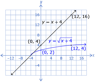
How does the graph of a function compare to the graph of the square root of the function? Compare the graphs for the functions y = x + 4 and ![]()
- Fill in the table of values. Create a graph using the values.
x y = x + 4 −6 −4 −3 0 5 12 -
Fill in the table of values. Create a graph using the values on the same grid that you graphed y = x + 4.
x 
−6 −4 −3 0 5 12 - Compare the two functions.
- State the domain and range of the two functions. Explain why you think they are different.
- When y = 0 for the original function, y = 0 for the square root of the function. Why?
- When y = 1 for the original function, y = 1 for the square root of the function. Why?
- When y = 4 for the original function, y = 2 for the square root of the function. Why?
![]() Save your responses in your course folder.
Save your responses in your course folder.
Share 1
With a partner or group, discuss the following question based on your graphs created for Try This 1:
Identify a pattern between the coordinates (x, y) of the first function y = x + 4 and the coordinates of the second function ![]()
![]() If required, save a record of your discussion in your course folder.
If required, save a record of your discussion in your course folder.
1.5. Explore
Module 2: Radical Functions
Explore
In Try This 1 you compared the graphs of y = x + 4 and ![]() You may have noticed that the mapping
You may have noticed that the mapping ![]() shows the correspondence between points on the first graph and those points on the second graph.
shows the correspondence between points on the first graph and those points on the second graph.
What other patterns do you see when you compare the original function y = x + 4 and the square root of the original function ![]()
In Try This 2 you will compare a given function to the square root of the given function.
Try This 2
Use Visualizing Square Root to compare a function f(x) and the square root of that function ![]()

Comparison 1 has been done for you as an example.
Comparison 1: Compare the functions f(x) = −x + 1 and ![]()
Step 1: Select the linear function in Visualizing Square Root.
Step 2: Use the sliders to set a to −1 and b to 1.
Step 3: Select the "Show Square Root" box and compare the two graphs. Record your observations in a table.
Solution
| f(x) = –x + 1 | ||
| Domain | {x|x ∈ R} | {x|x ≤ 1, x ∈ R} |
| Range | {y|y ∈ R} | {y|y ≥ 0, y ∈ R} |
| Invariant Point(s) |
(1, 0) and (0, 1) | |
| Sketch/Image of Both Functions | 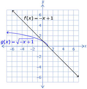 |
|
Comparison 2: Compare the functions f(x) = 0.5x − 1 and ![]()
Step 1: Change a to 0.5 and b to −1.
Step 2: Record your observations in a table similar to the following one.
| f(x) = 0.5x − 1 | ||
| Domain | ||
| Range | ||
| Invariant Point(s) | ||
| Sketch/Image of Both Functions | ||
Comparison 3: Compare the functions f(x) = x2 − 1 and ![]()
Step 1: Change the function to quadratic.
Step 2: Change a to 1, h to 0, and k to −1.
Step 3: Record your observations in a table similar to the following one.
| f(x) = x2 − 1 | ||
| Domain | ||
| Range | ||
| Invariant Point(s) | ||
| Sketch/Image of Both Functions | ||
Comparison 4: Compare the functions f(x) = 3x2 + 4 and ![]()
Step 1: Change a to 3, h to 0, and k to 4.
Step 2: Record your observations in a similar table.
| f(x) = 3x2 + 4 | ||
| Domain | ||
| Range | ||
| Invariant Point(s) | ||
| Sketch/Image of Both Functions | ||
- Look at the location of the invariant points. Is there a pattern? Why are the invariant points located where they are?
- How do the domains compare? Why are there differences?
- How do the ranges compare? Explain the differences.
- Refer to the sketches of each comparison. What happens to the value of
 as the value of f(x) changes? Use the following table to summarize the common patterns you observed for all four comparisons.
Value of f(x)
(original graph)When the y values are less than 0
(f(x) < 0)When the y value is 0
(f(x) = 0)When the y values are between 0 and 1
(0 < f(x) < 1)When the y value is 1
(f(x) = 1)When the y values are greater than 1
(f(x) > 1)Value of 
![]() Save your responses in your course folder.
Save your responses in your course folder.
Share 2
With a partner or group, discuss the following questions based on your graphs created in Try This 2:
Based on the patterns you identified in Try This 2, create a method you could use to graph the square root of any function.
![]() If required, save a record of your discussion in your course folder.
If required, save a record of your discussion in your course folder.
An invariant point is a point on a graph that remains the same after a transformation is applied to the graph.
1.6. Explore 2
Module 2: Radical Functions
During Try This 1 and Try This 2, you began to notice patterns between the graphs of y = f(x) and ![]() Do these patterns help you graph the square root of any function?
Do these patterns help you graph the square root of any function?
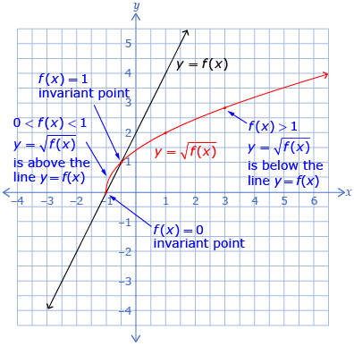
Your chart from Try This 2, which summarizes the patterns between the graphs of y = f(x) and ![]() , may or may not look similar to the following chart. However, the patterns should be similar. This chart arranges the patterns by the value of the original function, y = f(x), and the effect on the graph of the square root of the function,
, may or may not look similar to the following chart. However, the patterns should be similar. This chart arranges the patterns by the value of the original function, y = f(x), and the effect on the graph of the square root of the function, ![]()
| f(x) | f(x) < 0 | f(x) = 0 | 0 < f(x) < 1 | f(x) = 1 | f(x) > 1 |
Note: Take the square root of the y-values of y = f(x), and the range must be positive. |

Based on the patterns you have seen throughout Lesson 2, you will see how to graph ![]() when given the graph y = f(x). Go to Graphing the Square Root of a Function.
when given the graph y = f(x). Go to Graphing the Square Root of a Function.

Self-Check 1
Complete question 4 on page 87 of the textbook. Answer
1.7. Explore 3
Module 2: Radical Functions
In Try This 1 and Try This 2 you discovered some of the patterns between the domain and range of y = f(x) and ![]()
The domains of the square root functions are restricted in the areas of the original graph where y < 0. That is, any portion of the original graph that lies below the x-axis will not appear in the graph of the square root function. The range is restricted because the square roots of negative values are not real numbers. As a result, the range contains only values that are greater than or equal to zero.
You will now examine methods to graphically or algebraically compare the domains and ranges of a function and its square root.
Read “Example 2” on pages 82 and 83 of the textbook. Note the following:
- Method 1 uses technology to graph and then compare domains and ranges.
- Method 2 uses algebra to identify the x-intercepts, y-intercept, and the maximum or minimum value of the original function. You then determine the corresponding key points on the graph of
 by taking the square root of the original function’s maximum or minimum value. If there are x-intercepts, these intercepts stay the same. The domain and range can then be determined by using the key points.
Self-Check 2
Complete questions 5.b. and 5.c. and questions 6.b. and 6.c. from “Practise” on page 87 of the textbook. Answer
You have graphed f(x) and ![]() when the equations are given to you. What happens if you are only given a graph of y = f(x)? Could you graph
when the equations are given to you. What happens if you are only given a graph of y = f(x)? Could you graph ![]() from a graph of y = f(x)?
from a graph of y = f(x)?
Review “Example 3” on page 84 of the textbook.
Self-Check 3
- Complete “Your Turn” on page 85. Answer
- Complete questions 8.a. and 8.c. and question 11 on page 87. Answer
1.8. Connect
Module 2: Radical Functions
Complete the Lesson 2 Assignment that you saved in your course folder at the beginning of the lesson. Show work to support your answers.
![]() Save your responses in your course folder.
Save your responses in your course folder.
Project Connection
You are now ready to apply your understanding of the relationship between a function and the square root of the function. Go to your Module 2 Project: Pendulums, and complete Part 2: Square Root of a Function.
1.9. Lesson 2 Summary
Module 2: Radical Functions
Lesson 2 Summary
In this lesson you looked at the graph of ![]() when given the graph of y = f(x). You can use the values from the function f(x) to predict the values of the function
when given the graph of y = f(x). You can use the values from the function f(x) to predict the values of the function ![]() The y-values of the points of
The y-values of the points of ![]() are the square roots of the y-values of the points on the original function y = f(x).
are the square roots of the y-values of the points on the original function y = f(x).
In terms of mapping: ![]() so
so ![]() The invariant points occur when f(x) = 0 and f(x) = 1 because the square root of 0 is 0 and the square root of 1 is 1. The domain of
The invariant points occur when f(x) = 0 and f(x) = 1 because the square root of 0 is 0 and the square root of 1 is 1. The domain of ![]() are the x-values of f(x) for which f(x) is greater than or equal to zero. The range of
are the x-values of f(x) for which f(x) is greater than or equal to zero. The range of ![]() are the y-values in the range of f(x) for which f(x) is defined.
are the y-values in the range of f(x) for which f(x) is defined.
| f(x) | f(x) < 0 | f(x) = 0 | 0 < f(x) < 1 | f(x) = 1 | f(x) > 1 |
Note: Take the square root of the y-values of y = f(x), and the range must be positive. |
Some of the key lesson points are highlighted on the following graph.
In Lesson 3 you will study how the graphs of radical functions can help solve radical equations.