Lesson 3

1. Lesson 3

1.4. Explore 2

Mathematics 20-2 Module 4

Module 4: Statistical Reasoning

Normal distributions play a very important role in statistics. Many phenomena generate data distributions that are very well approximated by a normal distribution such as height, blood pressure, and scores on aptitude tests.

Recall that with a normal distribution, half the data is to the left of the line of symmetry (mean) and half the data is to the right of the line of symmetry. So, the total area under the normal curve and above the horizontal axis is equal to 1—this represents all of the data.

Try This 2

Use the interactive applet Area Under a Normal Curve to investigate the properties of a normal distribution.

Answer the following questions about normal distributions.

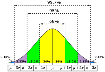
What percentage of data is within one standard deviation of the mean?
What percentage of data is within two standard deviations of the mean?
What percentage of data is within three standard deviations of the mean?
What percentage of data is beyond three standard deviations of the mean?

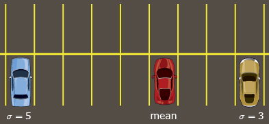
One way to help you visualize mean and standard deviation is to think about a parking lot. Suppose that you are meeting some friends at the mall. You all end up parking in the same row of stalls. Your one friend is parked five stalls away from you. Your other friend is parked three stalls away from you. The mean is your point of reference (i.e., your parking stall) and the standard deviation is how far away you are from the parking stalls where your friends are parked (i.e., five parking stalls and three parking stalls). So, your friend who is parked in the blue car is five standard deviations away from you, while the yellow car is three standard deviations away from you.

This illustration is of a row of parking stalls. A red car and a blue car are parked five stalls away from each other. A yellow is parked three stalls away from the red car.

In Try This 2, you learned that you can determine the percentage of the data that falls between any two whole number standard deviations on the normal curve using the rule of 68-95-99.7. That is, 99.7% of the data is within three standard deviations of the mean. So 0.3% of the data is more than three standard deviations from the mean.

This illustration shows a normal curve. About 68% of the data is within one standard deviation of the mean. About 95% of the data is within two standard deviations of the mean. About 99.7% of the data is within three standard deviations of the mean. About 0.3% of the data is more than three standard deviations away from the mean.

Because of its specific properties, the normal curve can be used to determine the likelihood that a certain event will occur. In other words, if you know that data is normally distributed, you can begin to look at what values you can expect to get in the future.

Read “Example 2: Analyzing a normal distribution” on pages 273 and 274 of your textbook. As you work through the example, think about how Jim uses the properties of a normal distribution to estimate the number of adult male dogs that will be within a specific weight interval.

Then read “Example 3: Comparing normally distributed data” on pages 275 and 276 of your textbook. As you complete the example, think about the factors that impact the shape of the normal curve. When the women added the weight of their baseballs and medals to their luggage, what changed in the data? Was it the mean? Was it the standard deviation?