Lesson 3
1. Lesson 3
1.5. Explore
Module 4: Polynomials
Explore
What you may have concluded in Share 1 is that linear regression is not appropriate for the bouncing ball data for two reasons:
- Graphical: The data is clearly not linear as the y-coordinates increase and then decrease.
- Contextual: After the ball goes up, it must come down—a process that can’t be modelled with a straight line.
The curve you created in Try This 1 is quadratic. As with linear data, spreadsheets and graphing calculators can perform quadratic regressions.
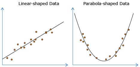
Linear regressions can be used with linear-shaped data. Quadratic regressions can be used with parabola-shaped (U) data.
When using a graphing calculator, the quadratic regression command is usually found in the same menu as linear regression.
The quadratic regression equation for the bouncing ball data calculated using a graphing calculator is y = −9.79x2 + 10.01x, where x is time in seconds and y is height in metres.
Notice that function matches trend of the data.
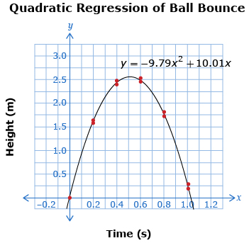
A regression equation that approximates the data can be used to determine how long the ball is in the air. Since the ball starts on the ground at time zero, the time it lands for the second bounce will be equal to the time it is in the air.
The ground is at height y = 0, so substituting 0 into the equation results in the following equation to be solved:
0 = −9.79x2 + 10.01x
The right side of this equation can factored:
![]()
By the zero product factor property:
or
Sometimes a quadratic equation cannot be solved by factoring. In these cases, the quadratic formula can be used:
The first answer, 0 s, corresponds to the first bounce. The second answer, 1.02 s, corresponds to the second bounce and the length of time that the ball is in the air.
Read “Example 1” on pages 308 to 310 of your textbook. Pay attention to the similarities between how a quadratic regression is used in this example and how linear regressions were used in the last lesson.
Self-Check 1
Complete questions 1, 3, 6, and 7 on pages 313 to 315 of your textbook. Answers