Lesson 3

In Try This 3, you saw that the cubic regression equation sometimes predicts unrealistic values and that you need to be careful when using a model to make predictions. Typically, interpolation (predicting a value within the data) is much more reliable than extrapolation (predicting a value outside the data).

Just as in the egg example, you may have noticed that solving the equation 3 = −0.0014x3 + 0.064x2 − 0.6399x + 11.7298 can be done by graphing both sides of the equation and finding the intersection.

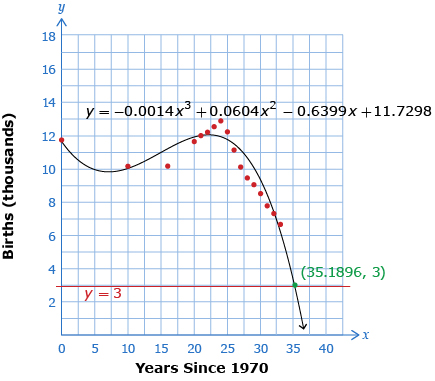
The graphs of y = −0.0014x3 + 0.064x2 − 0.6399x + 11.7298 and
y = 3 intersect at (35.1896, 3). Therefore, 35.1896 is a solution to the equation 3 = −0.0014x3 + 0.064x2 − 0.6399x + 11.7298.