Lesson 4
| Site: | MoodleHUB.ca 🍁 |
| Course: | Math 20-2 SS |
| Book: | Lesson 4 |
| Printed by: | Guest user |
| Date: | Monday, 29 December 2025, 11:41 PM |
Description
Created by IMSreader
1. Lesson 4
Module 4: Statistical Reasoning
Lesson 4: Z-Scores
Focus

© angelo.gi/21786273/Fotolia
Over the last three months, a cookie company has had an increase in the number of cookies that are broken and, therefore, need to be thrown out. In other words, these cookies do not meet the minimum quality standard. The more cookies that are thrown out before packaging, the less money the company will make.
The company decides to compare products produced at its four manufacturing facilities to see if the problem is occurring at only one facility or if the problem is occurring at more than one facility. If a problem is found in any facility, the company will then compare products produced by different work shifts to see if the problem is due to human error. Otherwise, if it doesn’t appear to be the fault of one work shift, the equipment needs to be examined for faults.
The normal curve for each of the manufacturing facilities and work shifts will be unique. Each data set will have its own mean and standard deviation. It is likely that the particular data value that the company wants to examine—in this case, the acceptable number of broken cookies—is not exactly one, two, or three standard deviations away from the mean. The company will need another way to analyze the data to help make good business decisions.
In this lesson you will learn about another tool that can be used to compare data, make predictions, and solve problems when dealing with normally distributed data.
This lesson will help you answer the following critical questions:
- How can two or more different normally distributed data sets be compared?
- How can the area under a normal curve be determined for values that are not exactly one, two, or three standard deviations away from the mean?
Assessment
- Lesson 4 Assignment
All assessment items you encounter need to be placed in your course folder.
![]() Save a copy of the Lesson 4 Assignment to your course folder.
Save a copy of the Lesson 4 Assignment to your course folder.
Materials and Equipment
- calculator
1.1. Discover
Module 4: Statistical Reasoning
Discover
Share 1

Photodisc/Thinkstock
Avery and Zachary are in different math classes. Avery’s math mark is 77%. Zachary’s math mark is 78%.
With a partner, discuss whether you can tell who is demonstrating a greater understanding in their math course based on their marks. How would you know? Can you apply your understanding of normal curves to help you decide?
1.2. Explore
Module 4: Statistical Reasoning
Explore
In Share 1 you and your partner may have determined that in order to meaningfully compare the two math marks, you need more information. At first glance, it appears that a mark of 78% is better than a mark of 77%. However, since these marks are so close, is there a better way to determine which student is demonstrating a greater understanding of math? For instance, if you knew the mean and standard deviation of each class, you could do a sketch of a normal curve for each class.
Suppose you were given the following information about Avery and Zachary’s math classes.
| Avery’s Class | Zachary’s Class |
| μ = 75.5% | μ = 76.5% |
| σ = 2.0% | σ = 2.5% |
The normal curves for each class might look something like the following.
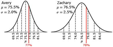
The normal curves might give you an idea of who is demonstrating a greater understanding in math. The student that is the farthest to the right on the curve would have demonstrated the greatest understanding. However, the answer might not be clear. You are comparing two very similar yet different normal curves. Because they are so similar, deciding which which mark is farther to the right may be difficult.
You and your partner may have thought about comparing the two math marks on the same normal curve; but, you can’t use the same normal curve unless the mean and the standard deviation are the same. In order to do this, you would need a way to standardize the math marks to fit on a common normal distribution. Then you could determine how many standard deviations each mark is away from the mean.
z-score: a measure of the number of standard deviations a particular data value is above or below the mean
standard normal distribution: a normal distribution that has a mean of zero and a standard deviation of one
—From CANAVAN-MCGRATH ET AL. Principles of Mathematics 11,
©2012 Nelson Education Limited. Reproduced by permission.
There is a way to standardize the marks! A z-score can be used to compare Avery and Zachary’s marks on the same normal distribution. A z-score is a measure of the number of standard deviations a particular data point is away from the mean on a standard normal distribution. A standard normal distribution is a normal distribution with a mean of zero and a standard deviation of one.
From CANAVAN-MCGRATH ET AL. Principles of Mathematics 11, © 2012 Nelson Education Limited. Reproduced by permission.
Any data point, x, from a normal distribution is a certain number of standard deviations away from the mean. This can be represented by the equation ![]() where z represents the z-score (i.e., the number of standard deviations the data point is away from the mean). A positive z-score means that the data value is above the mean. A negative z-score means that the data value is below the mean.
where z represents the z-score (i.e., the number of standard deviations the data point is away from the mean). A positive z-score means that the data value is above the mean. A negative z-score means that the data value is below the mean.
Look at the marks in Zachary’s math class again. You know that μ = 76.5% and σ = 2.5%. If you were in Zachary’s math class and you had a mark of 79%, it is exactly one standard deviation above the mean (76.5 + 2.5 = 79). If your mark was 69%, you can see that it is exactly three standard deviations below the mean (76.5 − 2.5 − 2.5 − 2.5 = 69).
To calculate a z-score that is not so easy to see, use this formula:
![]()
For instance, you would use the formula to calculate a z-score that is not exactly one, two, or three standard deviations from the mean.
Recall that Avery has a math mark of 77% and Zachary has a math mark of 78%. The mean mark for Avery’s class is 75.5% with a standard deviation of 2%. The mean mark for Zachary’s math class is 76.5% with a standard deviation of 2.5%. You can compare how far above or below the mean the marks are by calculating z-scores for them.
| Avery: | Zachary: |
 |
 |
So, Avery’s math mark is 0.75 standard deviations above the mean, and Zachary’s is 0.6 standard deviations above the mean. Each student’s z-score is shown on the following standard normal distribution.

So, when the marks are standardized, Avery’s mark is farther to the right on the standard normal distribution, with a z-score of 0.75, as compared to Zachary’s z-score of 0.6. Therefore, Avery actually has the better mark.
Read “Example 1: Comparing z-scores” on pages 283 to 284 of the textbook. As you work through the example, notice the importance of standardizing Hailey’s run times in order to get a true comparison.
Self-Check 1
- What z-score corresponds with each location on a standard normal curve?
- 1 standard deviation above the mean
- 1 standard deviation below the mean
- equal to the mean
- 1.5 standard deviations above the mean
- 3.2 standard deviations below the mean
- 1 standard deviation above the mean
- Complete “Check Your Understanding” question 1 on page 292 of the textbook. Answer
- Complete “Practising” question 10 on page 292 of the textbook. Answer
1.3. Explore 2
Module 4: Statistical Reasoning
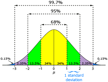
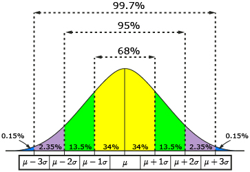
In Lesson 3 you learned that the 68%-95%-99.7% property of normal distributions could be used to make estimates about data that is exactly one, two, or three standard deviations away from the mean. But as you have seen so far in this lesson, the data value you need may not be exactly one, two, or three standard deviations away from the mean.
There are an infinite number of standard deviations that a data value can be above or below a mean. For instance, a data value could be 1.56, 0.25, or 3.02 standard deviations above the mean. A data value could also be 2.79, 0.5, or 3.58 standard deviations below the mean.
Consider the following situation.
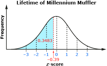
A muffler company makes and supplies the car industry with mufflers. The lifetime of the company’s best-selling muffler, the Millennium Muffler, is normally distributed with a mean of 7.2 years and a standard deviation of 1.8 years. The company wants to determine what percentage of its Millennium Mufflers will last less than 6.5 years.
To visualize the situation, you can sketch the normal distribution for the lifetime of the Millennium Muffler.
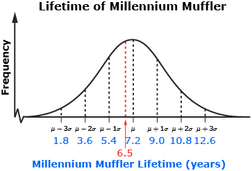
A lifetime of 6.5 years is between the mean and one standard deviation below the mean. Z-scores can be used when you are dealing with normally distributed data values that are not exactly one, two, or three standard deviations away from the mean.
The z-score formula can be used to determine the z-score for a muffler life of 6.5 years.
A muffler life of 6.5 years is about 0.39 standard deviations below the mean. A z-score of −0.39 is shown on a standard normal curve. The company wants to determine the percentage of Millennium Mufflers that will last less than 6.5 years. This is equivalent to the area under the curve to the left of −0.39 on the standard normal curve.

z-score table: a table that displays the fraction of data with a z-score that is equal to or less than a given value in a standard normal distribution
— From CANAVAN-MCGRATH ET AL. Principles of Mathematics 11,
© 2012 Nelson Education Limited. Reproduced by permission.
A z-score table can be used to determine the percent of data that is equal to or less than (i.e. to the left of) any given z-score in a standard normal distribution.
A z-score table can be found on pages 580 and 581 of the textbook. Or you can go to Z-Score Table to see an example.
When you read a z-score table, you begin by rounding your z-score to two decimal places. Locate the z-score up to the first decimal place in the left-hand column of the table. Then find the second decimal place in the row across the top of the table. Where the row and column intersect, you will find your z-score value. For a z-score of −0.39, find the −0.3 row and then the 0.09 column on the z-score table.
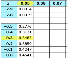
From CANAVAN-MCGRATH ET AL. Principles of Mathematics 11,
© 2012 Nelson Education Limited. Reproduced by permission
The value in the table is 0.3483. This is the fraction of the area under the curve that is to the left of a z-score of −0.39. This means that about 34.8% of Millennium Mufflers will have a lifetime of 6.5 years or less.
1.4. Explore 3
Module 4: Statistical Reasoning
The statistics function for normal distributions on a calculator can also be used to determine the percent of data that is less than a specific data value. To access the statistical function for normal distribution on your calculator, you may press ![]()
![]() and then select “2: normalcdf(.”
and then select “2: normalcdf(.”
![]()
You will now enter four values separated by commas. The first value that is entered is the lower bound. This is the value that would be on the furthest left-hand side of the curve. In the example of the muffler, the least amount of time a muffler could last is zero years. The next value is the upper bound, or 6.5 years. Finally, the mean and standard deviation are entered. So, the area under the normal distribution that is less than a value of 6.5 years is 0.348 647 533 9 or 34.9%.

When calculating the area under a curve, you may find that you get slightly different results depending on whether you use the z-score table or the statistics function for normal distribution on your calculator. The z-score table uses a rounded z-score for identifying the fraction of data that is to the left of a particular z-score.
Self-Check 2
1.5. Explore 4
Module 4: Statistical Reasoning
![]()
Let’s consider the muffler company again. Suppose the muffler company wanted to determine how many Millennium Mufflers had a lifetime of at least 9.25 years.
Try This 1
If 10 000 mufflers are produced, how many will last at least 9.25 years? Use the interactive applet Lifetime of a Millennium Muffler to determine what percentage of Millennium Mufflers should last at least 9.25 years.

muffler: iStockphoto/Thinkstock
Self-Check 3
Complete “Practising” question 7 on page 292 of your textbook. Answer
1.7. Lesson 4 Summary
Module 4: Statistical Reasoning
Lesson 4 Summary
Z-scores can be used to solve problems when you are dealing with normally distributed data values that are not exactly one, two, or three standard deviations away from the mean. Z-scores and the standard normal distribution can also be used to compare different sets of normally distributed data.
Different strategies can be used to determine the percent of data that is less than or greater than a given value in a normal distribution. Whether you use a z-score table or a graphing calculator, it is important to always keep in mind what area under the curve you are dealing with. Ask yourself this: does the situation refer to the area under the curve to the left or the right of the data value or z-score?
In Lesson 5 you will continue to solve problems using z-scores.