Lesson 8
| Site: | MoodleHUB.ca 🍁 |
| Course: | Math 20-1 SS |
| Book: | Lesson 8 |
| Printed by: | Guest user |
| Date: | Thursday, 4 December 2025, 2:15 AM |
Description
Created by IMSreader
1. Lesson 8
Module 4: Quadratic Equations and Inequalities
Lesson 8: Solving Quadratic Inequalities in One Variable
Focus

iStockphoto/Thinkstock
If you had unlimited resources to design a community that minimized its impact on the environment, what would your design look like? What kind of materials would be used to construct the buildings in your community? How would you reduce carbon emissions from transportation?
Building communities that fit into the environment isn’t a new idea. The Anisazi of the southwestern United States built communities using local materials. Similar communities can be found in Mali and in the city of Petra, in Jordan. These buildings used ideas that environmental designers are still using today. Building into a cliff provides thermal stability—have you seen homes that seem to be built underground except for one wall? Have you ever opened a window after a hot summer day to get the cooler evening air into a room? Search for “environmental city design” to find some striking images and interesting ideas.
In this lesson you will study quadratic inequalities in one variable. You will learn how to solve these inequalities by graphing and by algebraic methods. You will also model and solve problems with quadratic inequalities, including one that deals with a special type of eco-friendly construction material.
Outcomes
At the end of this lesson you will be able to
- determine the solution of a quadratic inequality in one variable using a variety of strategies
- represent and solve a problem that involves a quadratic inequality in one variable
- interpret the solution to a problem that involves a quadratic inequality in one variable
Lesson Questions
You will investigate the following questions:
- What principle is common to all strategies for solving quadratic inequalities?
- How can you tell when a problem can be modelled by a quadratic inequality in one variable?
Assessment
Your assessment may be based on a combination of the following tasks:
- completion of the Lesson 8 Assignment (Download the Lesson 8 Assignment and save it in your course folder now.)
- course folder submissions from Try This and Share activities
- additions to Module 4 Glossary Terms and Formula Sheet
- work under Project Connection
1.1. Launch
Module 4: Quadratic Equations and Inequalities
Launch
Do you have the background knowledge and skills you need to complete this lesson successfully? This section, which includes Are You Ready? and Refresher, will help you find out.
Before beginning this lesson you should be able to
- interpret inequality statements
- graph inequalities on number lines
- factor quadratic equations
- use the quadratic formula
1.2. Are You Ready?
Module 4: Quadratic Equations and Inequalities
Are You Ready?
Inequalities may often be satisfied by more than one set of values for the unknowns. For example, think of two numbers the product of which is positive. Did you think of two positive numbers, or did you choose two negative numbers? Sorting through the various possibilities is an important skill in solving quadratic inequalities. The following questions will give you a taste of what’s to come!
Complete these questions. If you experience difficulty and need help, visit Refresher or contact your teacher.
- If ab > 0, which of the following statements could be true?
- a > 0, b > 0
- a > 0, b < 0
- a < 0, b > 0
- a < 0, b < 0
Answer
- If ab ≤ 0, which of the following statements could be true?
- a ≥ 0, b ≥ 0
- a ≥0, b ≤ 0
- a ≤ 0, b ≥ 0
- a ≤ 0, b ≤ 0
Answer
- Graph each of the inequalities on a number line.
- Solve each quadratic equation by factoring.
- Solve each quadratic equation by using the quadratic formula.
How did the questions go? If you feel comfortable with the concepts covered in the questions, move on to Discover. If you experienced difficulties, use the resources in Refresher to review these important concepts before continuing through the lesson.
1.3. Refresher
Module 4: Quadratic Equations and Inequalities
Refresher
Use the following to review the Launch topics you experienced difficulties with in the Are You Ready? section.
Khan Academy (CC BY-NC-SA 3.0)
For more information about interpreting inequality statements, watch “Multiplying and Dividing Negative Numbers.”

Khan Academy (CC BY-NC-SA 3.0)
Also watch “Inequalities on a Number Line.”

The Inequality website reviews how to graph inequalities on a number line and has an applet at the bottom of the page to practise graphing more inequalities.
To review how to factor quadratic equations, you may find the following helpful:
- Use Solving Quadratic Equations: Factoring to review your factoring skills. Once you have selected Solving Quadratic Equations: Factoring, choose the Examples button, shaped like a puzzle piece, at the top of the page. Work through the examples provided.

- Go back to Lessons 2 and 4 of this module to review your factoring skills.

Use The Quadratic Formula: Problem Situations to review the use of the quadratic formula. After choosing The Quadratic Formula, select the Examples button, shaped like a puzzle piece, at the top of the page. Work through all four of the examples provided.
Go back to the Are You Ready? section and try the questions again. If you are still having difficulty, contact your teacher.
1.4. Discover
Module 4: Quadratic Equations and Inequalities
Discover

In this section, you will use an interactive applet to learn about quadratic inequalities.
Try This 1

Launch Quadratic Inequalities Explorer.
- Complete the Quadratic Inequalities Table as you work through the Quadratic Inequalities Explorer.
- Based on your observations recorded in the table from question 1, complete the following three statements using either above, below, or on.
- The points (yellow
 ) you identified for f(x) = 0 were _______the x-axis.
- The points (red
 ) you identified for f(x) < 0 were _____the x-axis.
- The points (green
 ) you identified for f(x) > 0 were ______the x-axis.
- The points (yellow
- What is the relationship between the inequality symbol of an inequality and the location of the solution set on the graph of the corresponding function?
- Graph the function y = x2 − 2x − 8.
- Based on the relationship you identified in question 3, where would you find the solutions to the inequality x2 − 2x − 8 ≥ 0?
![]() Save your work in your course folder.
Save your work in your course folder.
You will need to retrieve these results later in the lesson.
1.5. Explore
Module 4: Quadratic Equations and Inequalities
Explore

Olympic Games 2016 Rio de Janeiro Solar City Tower Concept Design Photo (Zurich: RFAA Architecture and Design, 2011.) Reproduced with permission.
The Solar City Tower in Brazil is an example of a structure that has been conceived with sustainability in mind. The symbol of the 2016 Olympic Games in Rio de Janeiro, the Solar City Tower will be seen by all those who arrive at the Games by air or water. The immense building is remarkable not only for its panoramic views, urban plaza, amphitheater, cafeteria, and shops, but also for its eco-friendly design that will feature a massive system for capturing solar energy. By day, the solar system will generate energy for the Olympic Village as well as some energy for the city of Rio. By night, a hydroelectric system of stored water and turbines will deliver energy to these same places. The Solar City Tower will be the home of the Olympic torch and will also feature a waterfall, which, according to its designers, symbolizes the “forces of nature.”
In this lesson you will use quadratic inequalities to model problems that deal with aspects of sustainable architecture, such as those exhibited by the Solar City Tower.
1.6. Explore 2
Module 4: Quadratic Equations and Inequalities
Solving Quadratic Inequalities in One Variable
A quadratic inequality in one variable can be written in any one of the following forms where a, b, and c are real numbers and a ≠ 0:
- ax2 + bx + c < 0
- ax2 + bx + c ≤ 0
- ax2 + bx + c > 0
- ax2 + bx + c ≥ 0
In Lesson 7, you explored inequalities in two variables. Quadratic inequalities in one variable may be solved by referring to the graphs of corresponding quadratic inequalities in two variables. The following inequalities in two variables correspond to the preceding inequalities in one variable:
- ax2 + bx + c < y
- ax2 + bx + c ≤ y
- ax2 + bx + c > y
- ax2 + bx + c ≥ y
In Discover you may have noticed something about the solution set of an inequality in one variable. The solution set corresponds to certain x-values of the graph of the corresponding inequality in two variables. Depending on the inequality, the chosen x-values will lie above, on, or below the x-axis. Quadratic inequalities in one variable can be solved by both graphical and algebraic methods.
The following example shows how you can solve quadratic inequalities in one variable by analyzing the graphs of corresponding functions in two variables. This example is based on the same question posed in Try This 1 question 4. Retrieve your work from Try This 1 so that you can compare your solution to the solution in the example.
Example
Solve x2 − 2x − 8 ≥ 0.
Solution
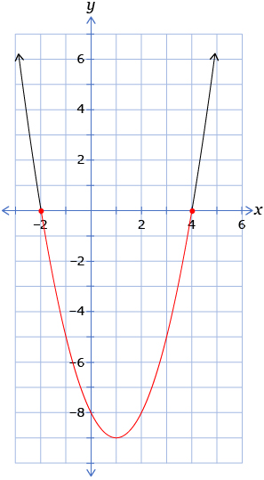
Graph the corresponding function y = x2 − 2x − 8.

The problem asks for the solutions to x2 − 2x − 8 ≥ 0. Since the function that the graph represents is y = x2 − 2x − 8, you need to determine where y ≥ 0. You can do this by identifying the points on the graph where the y-coordinate is greater than or equal to 0. These points are on and above the x-axis, shown in red on the following graph.
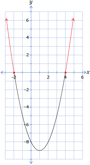
You can report the solution as the domain of the parts of the graph highlighted in red. The domain is all real values less than or equal to –2 or greater than or equal to 4.
The solution set is {x | x ≤ − 2 or x ≥ 4, x ∈ R}.
Compare your solution from Try This 1 to the solution in the example. Make any necessary revisions to your work.
Turn to “Example 1” on pages 478 to 479 of the textbook. You are asked to solve a different quadratic inequality. Work your way through Method 1 only. Ask yourself the following questions as you work through the method:
- What other ways could you report the solution?

- How can you sketch the graph of a quadratic function when the function is written in standard form?
Self-Check 1
Use the following information to answer the next two questions.
- What is the solution to the quadratic inequality −5x2 + 20x − 15 < 0?
- x < 1
- x > 3
- 1 < x < 3
- x < 1 or x > 3
- What is the solution to the quadratic inequality −5x2 + 20x − 15 ≥ 0?
- 1 < x < 3
- 1 ≤ x ≤ 3
- x < 1 or x > 3
- x ≤ 1 or x ≥ 3
- Select the choice or choices for which the stated value of x is a solution to the given inequality.
- x = 0 for −x2 − 5x + 1 < 0
- x = −3 for x2 + x − 6 > 0
- x = 12 for −0.5x2 + 4x + 17 ≥ 0
- x = 1 for 2x2 − 7x + 3 ≤ 0
- The solution to the inequality 2x2 − 7x ≤ 3 is found in the interval a ≤ x ≤ b. What is the sum of a and b to the nearest tenth? Answer
1.7. Explore 3
Module 4: Quadratic Equations and Inequalities
Roots and Test Points Method
The next part of the lesson will focus on algebraic methods of solving quadratic inequalities. The first of these methods is based on determining the roots of the equation corresponding to the quadratic inequality. These roots are known as critical values and are used to divide the domain of real numbers into intervals.
Try This 2

Launch the Solving Inequalities 1 interactive lesson. Select Solving Inequalities 1, and then select the tutorial icon at the top of the window. Choose Solving Quadratic Inequalities in One Variable.
As you work through the interactive lesson, respond to the following questions.
- How are the critical values along the number line related to the quadratic inequality?
- How are test points selected?
- Why is only one test point selected for each interval?
![]() Save your responses to your course folder.
Save your responses to your course folder.
Turn to “Example 3” on page 482 of the textbook to see how you can use the roots and test points approach to solve a quadratic inequality that cannot be factored. As you work through the example, look for the answers to the following questions:
- Why should you rewrite the inequality so that one side is equal to 0?

- What can be done with quadratic expressions that are not factorable?
- What strategies can you use to make exact values easier to work with?
You may want to refer to these answers when you tackle your lesson assignment.
Self-Check 2
Turn to page 485 in the textbook to practise using the roots and test points method for solving quadratic inequalities. Complete question 4. Answer
1.8. Explore 4
Module 4: Quadratic Equations and Inequalities
Sign Analysis
Another algebraic approach is based on analyzing the signs of the factors in the quadratic expression.
Try This 3

Turn to “Example 2” on pages 480 and 481 in the textbook. This example shows how you can use each of the algebraic methods that you have learned so far to solve a quadratic inequality of the form ax2 + bx + c < 0 where a < 0. You will benefit from reviewing both methods, but you will also find it helpful to see how a negative leading coefficient, when a < 0, is handled. As you work through the example, answer the following questions:
- How could you choose test points so that it would be easier to evaluate the sign of the function?

- How are negative constant factors dealt with?
Case Analysis
A third approach that can be used to solve quadratic inequalities is carried out by first identifying the conditions under which a quadratic inequality is true. The conditions are identified by analyzing the possible sign of each factor. A number line can then be used to determine when those conditions will be satisfied.
Try This 4

Launch the interactive lesson titled Case Analysis: Another Strategy for Solving Quadratic Equations.
Turn to “Example 1” on page 478 of the textbook. Work your way through Method 1 only. Ask yourself the following questions as you work through the method:
- How does the solution process change when the inequality symbol is ≤ or ≥ compared to < or >?
- How is the reasoning process that leads to the solution interval in the example similar to the reasoning process used in the Case Analysis interactive lesson?
Self-Check 3
Turn to page 485 of the textbook to practise solving quadratic inequalities using the sign analysis and case analysis methods. Complete questions 5.a., 5.c., 6.b., and 6.d. You may wish to save your rough work in your course folder for future reference. If you make a mistake, don’t worry! Just give it another try. Answer
1.9. Explore 5
Module 4: Quadratic Equations and Inequalities
Modelling Problems with Quadratic Inequalities
The phrase “carbon footprint” refers to the amount of greenhouse gases produced through such activities as manufacturing a product or constructing a house. A carbon-neutral home or a zero-carbon home is a home where the net amount of carbon emissions from energy consumption over one year is 0. Such homes may be outfitted with geothermal heating and cooling features, solar energy panels, water conservation properties, and carbon-neutral building materials. Such homes are said to have a carbon-neutral footprint.

© The Freestead Project. Used with permission.
Try This 5
Suppose the following graph shows the housing-price-to-construction-cost ratio of carbon-neutral homes for a Canadian city. The equation relates the housing-price-to-construction-cost ratio, y, of the number of years, x, since the year 2000. Here, 0 ≤ x ≤ 12.
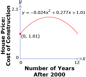
- Between what years was the housing-price-to-construction-cost ratio less than 1.5? Write an inequality that models the problem.
- Solve the inequality. Explain the strategy you used.
- The solution to the inequality from question 2 should be in the form of an interval. Interpret this interval.
![]() Save your responses in your course folder.
Save your responses in your course folder.
Share 1
With a classmate, compare your answers to Try This 5. Discuss the following questions.
- What algebraic strategy or strategies may be appropriate to apply to this problem?
- How many different ways could you solve this problem graphically?
- How can this problem be modelled as a linear-quadratic system of equations?
![]() Save your responses in your course folder.
Save your responses in your course folder.
1.10. Explore 6
Module 4: Quadratic Equations and Inequalities
Turn to “Example 4” on page 483 of the textbook to find another example of how quadratic inequalities can be applied to a problem involving the time a baseball is in flight. Confirm your understanding of the problem by determining why the inequality must be greater than zero in this instance.
Self-Check 4
Complete questions 10, 12, and 13 on pages 485 and 486 in the textbook. Answer
1.11. Connect
Module 4: Quadratic Equations and Inequalities
Connect
Lesson 8 Assignment
Open your copy of the Lesson 8 Assignment, which you saved in your course folder at the start of this lesson. Complete the assignment.
![]() Save your work in your course folder.
Save your work in your course folder.
Project Connection

© wong yu liang/29976438/Fotolia
Go to Module 4 Project: Imagineering. Complete Step 6: Expansion.
![]() Save your work in your course folder.
Save your work in your course folder.
Going Beyond
Part A
In this lesson you learned several strategies for solving quadratic inequalities. You can extend these strategies to the solution of polynomial inequalities.
The following graph represents the cubic function f(x) = 0.08(x + 5)(x + 2)(x – 7).
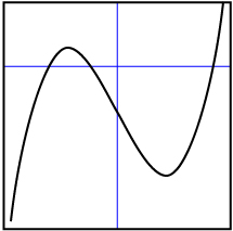
Apply at least two of the strategies you used in this lesson to solve the inequality 0.08(x + 5)(x + 2)(x − 7) ≤ 0.
![]() Save your work in your course folder.
Save your work in your course folder.
Part B: Calculate Your Carbon Footprint
You can determine your impact on the environment by calculating your own carbon footprint. Search the Internet for “carbon footprint calculator.” Find a calculator that allows you to input information about your lifestyle and environmental practices. You can make a plan to improve your score by following environmentally friendly practices.
![]() Save your work in your course folder.
Save your work in your course folder.
1.12. Lesson 8 Summary
Module 4: Quadratic Equations and Inequalities
Lesson 8 Summary

© morganimation/12959959/Fotolia
In this lesson you investigated the following questions:
- What principle is common to all strategies for solving quadratic inequalities?
- How can you tell when a problem can be modelled by a quadratic inequality in one variable?
In this lesson you learned that quadratic inequalities in one variable can be solved in a number of different ways. Whether you solve quadratic inequalities in one variable graphically or algebraically, there is one principle that is common to them all. A quadratic inequality can be greater than 0 or less than 0, which means that the y-values are either positive or negative.
Therefore, regardless of the method you choose, you must determine solutions based on whether the y-coordinates in the solution are positive or negative. The following table summarizes how you determine the solution intervals based on signs.
| Strategy for Solving | How to Determine the Solution Interval(s) |
| Graphing | Look above the x-axis if f(x) > 0 or f(x) ≥ 0.
Look below the x-axis if f(x) < 0 or f(x) ≤ 0.
|
| Roots and Test Points | Use a test point from each interval to determine if the interval will yield positive or negative values of the function.
|
| Sign Analysis | Consider the signs of the factors at each interval. Select the solution interval(s) based on the signs of the product of the factors.
|
| Case Analysis | Consider what the signs of the factors could be in order to satisfy the inequality based on the following four possible cases:
Then graph each possible case to determine the solution intervals. |

You also modelled problems with quadratic inequalities in one variable. There are two conditions that are common to such problems. The first is that the situation can be represented by a quadratic function. The second is that the problem asks about points on the function that are greater than or less than a reference point.