Lesson 2
| Site: | MoodleHUB.ca 🍁 |
| Course: | Math 30-3 SS |
| Book: | Lesson 2 |
| Printed by: | Guest user |
| Date: | Monday, 10 November 2025, 5:57 AM |
Description
Created by IMSreader
1. Lesson 2
Module 3: Algebra
Lesson 2: Equation of a Line
Focus
Have you ever tried to bike up a steep hill? The steepness of an incline is measured using a grade. A grade is the ratio of the rise of an incline to its run. If a hill rises 100 m for every 1000 m of run, you would say the hill’s grade is ![]() or 0.1. Most road signs show the grade as a percent. Recall from Mathematics 20-3 that
or 0.1. Most road signs show the grade as a percent. Recall from Mathematics 20-3 that
![]()
Therefore, if the rise is 100 m and the run is 1000 m, the grade would be 10%, calculated as follows:
![]()
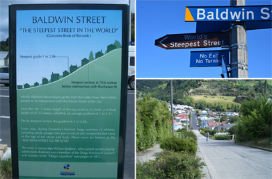
Left: Ullisan/flickr; top right: RabunWarma/flickr; bottom right: Ullisan/flickr.
All images used under Creative Commons Licence (2.0 Generic). Attribution-NoDerivs).
Have you ever noticed that the middle of the road is slightly higher than at the road’s curbs? This is because roads are built with at least a 1% grade so that water will run off to the sides of the road. When building wheelchair ramps the grade is not to exceed 1:12, or about 8.3%.
Baldwin Street in Dunedin, New Zealand, is the world’s steepest street, according to the Guinness Book of Records. The grade of Baldwin Street is approximately 35%. Do you think you could peddle up Baldwin Street?
Lesson Outcomes
At the end of this lesson you will be able to
- determine the slope from a pair of points, and then come up with the equation of a line
- create a table of values and be able to write a linear equation in the form

Lesson Questions
You will investigate the following questions:
- How does the equation of a linear function relate to the function’s graph?
- How are the properties of linear functions applied to studying and solving problems?
Assessment
Your assessment may be based on a combination of the following tasks:
- completion of the Lesson 2 Assignment (Download the Lesson 2 Assignment and save it in your course folder now.)
- course folder submissions from Try This and Share activities
- additions to Glossary Terms and Formula Sheet
Materials and Equipment
You will need
- calculator
- straight edge or ruler
- Grid Paper Template
1.1. Launch
Module 3: Algebra
Launch
Do you have the background knowledge and skills you need to complete this lesson successfully? Launch will help you find out.
Before beginning this lesson you should be able to
- find the slope of a line given two points
- solve for the unknown variable in a two-step equation
1.2. Are You Ready?
Module 3: Algebra
Are You Ready?
Complete these questions. If you experience difficulty and need help, visit Refresher or contact your teacher.
- Using the slope formula
 , find the slope of the line passing through (−1, 5) and (9, −5). Answer
 - Solve for the unknown in each of the following.
If you answered the Are You Ready? questions without difficulty, move to Discover.
If you found the Are You Ready? questions difficult, complete Refresher.
1.3. Refresher
Module 3: Algebra
Refresher

Screenshot reprinted with permission of ExploreLearning.
Work through the Solving Two-Step Equations interactive.
Go back to the Are You Ready? section and try the questions again. If you are still having difficulty, contact your teacher.
1.4. Discover
Module 3: Algebra
Discover

© Dwight Smith /9676362/Fotolia
Try This 1
A truck driver transports lumber from Grande Prairie to Calgary, Alberta. The driver’s map shows that the distance between Grande Prairie and Calgary is about 750 km. The driver knows that she can average 90 km/h, including stops. If she leaves Grande Prairie at 8:00 a.m., will she make it to Calgary by 4:00 p.m.?
- Complete a table of values like the one shown.
Time Travelled
Distance from Calgary (km)
0
750
1
660
2
570
3
4
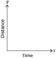
- Using your table of values, create a graph similar to the one shown. Connect the points with a straight line and make sure you extend the line to touch the horizontal axis. You can create a graph by hand, digitally with the use of a spreadsheet, or by using Graph Paper Template.
- Will the truck driver make it to Calgary before 4:00 p.m.? Explain your answer and determine the truck’s arrival time.
![]() Save your responses in your course folder.
Save your responses in your course folder.
Share 1
With a partner or in a group, share your strategy and responses. In your sharing session, consider the following discussion questions.
- What is the slope of your graph?
- What does the slope of your graph represent in the question?
- Why is the slope negative?
- What is the y-intercept of your graph?
- What does the y-intercept of your graph represent in the question?
- In this case, should the points be connected? Explain.
1.5. Explore
Module 3: Algebra
Explore

© Katrina Brown/16686740/Fotolia
Through your Share discussions, you may have discovered that there are a number of methods to determine whether the truck driver will arrive on time. You may have determined your answer by extending the table of values up to 8 h, by drawing the graph, or by creating and solving a direct linear equation. Regardless of the method you used, it is important that you are able to clearly and confidently support your answer through your shown work.
In the Discover activity the graph you constructed should have resembled the following graph:
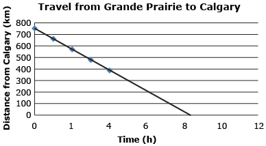
From the graph, you can clearly see the trip will take over 8 h, since the line crosses the x-axis between 8 and 9 h. As a result, you can confidently conclude that the truck will not arrive by 4:00 p.m.
To calculate the slope, choose two points on the line; for example (0, 750) and (4, 390). Apply the slope formula.
![]()
Substitute the values for x and y.
Since the vertical units are kilometres (km), and the horizontal units are hours , the slope is –90 km/h. This value represents the average speed of the truck. The slope is negative because the line is falling to the right (from the graph) or negative because the distance from Calgary is lessening by 90 km for every hour travelled.
The y-intercept is 750, and this relates to the initial distance from Grande Prairie to Calgary. In this case the points should be connected. This is because, for every hour or part thereof, the trucker is getting closer to Calgary.
Any linear relation can be described by the formula y = mx + b, where (x, y) represents any point on the line, m is the slope, and b is the y-intercept. The above linear relation can then be described as y = −90x + 750.
You noted from the graph that it would take over 8 h to make the trip to Calgary. To be more exact you could find the x-intercept, the place where the line touches the horizontal axis and is described by the point (x, 0). Substitute (x, 0) into the equation and solve for x.
The trip will take ![]() or 8 h and 20 min. The driver will arrive at approximately 4:20 p.m.
or 8 h and 20 min. The driver will arrive at approximately 4:20 p.m.
1.6. Explore 2
Module 3: Algebra
By now you may have found that any linear relation can be described using the standard linear equation y = mx + b, where m represents the slope of the line and b represents the y-intercept.
Notice that if the relation passes through the origin at point (0, 0), the equation can be reduced to y = mx. Equations that can be expressed as y = mx are direct linear relations.
Open Direct Linear Relations (y = mx) and move the slider to explore different values of m for y = mx.
Study and review “Example 1” and the solutions on pages 30, 31, and 32 of the textbook.
1.7. Explore 3
Module 3: Algebra
Partial linear relations have equations that can be expressed using y = mx + b. This type of equation also yields a straight line with slope m; however, the line passes through a y-intercept (0, b).
Open Partial Linear Relations (y = mx + b) and move the sliders to explore different values of m and b in y = mx + b.
Study and review the following examples and solutions in the textbook:
- “Example 2” on page 35
- “Example 3” on page 36
Self-Check 1
It is time to check your understanding of direct and partial linear relations. Give the following a try!
Salina is deciding on whether to join a local pickup hockey league or purchase a gym membership. The hockey league charges its players $7 per game. Whereas the gym membership charges a yearly fee of $210, plus $2 per visit. ![]()
- Write equations that represent the cost in relation to the number of outings for each option. Answer
- If Salina decides that she is able to attend 45 outings over 6 months, which option is least costly? Answer
- How many outings would result in the same cost for both options? In other words, how many times would Salina have to go to the gym or to play hockey in order for both options to cost the same amount?
 Answer
Self-Check 2
Add the following terms to your copy of Glossary Terms:
- x-intercept
- y-intercept
Add the following formulas to your copy of Formula Sheet:
- y = mx
- y = mx + b
1.8. Connect
Module 3: Algebra
Complete the Lesson 2 Assignment that you saved in your course folder at the beginning of the lesson. Show work to support your answers.
![]() Save your responses in your course folder.
Save your responses in your course folder.
Project Connection
You are now ready to apply your understanding of equations of linear relations to Module 3 Project: Household Water Conservation. Go to the Module 3 Project, and complete Part 2.
![]() Save your responses in your course folder.
Save your responses in your course folder.
1.9. Lesson 2 Summary
Module 3: Algebra
Lesson 2 Summary
In this lesson you looked at equations of linear relations.
Direct linear relations can be described using the equation y = mx. The graph of a direct linear relation will always be straight (linear) and will pass through the origin (0, 0).
Partial linear relations can be described using the equation y = mx + b. The graph of a partial linear relation will always be straight (linear). However, the graph will pass through the y-axis at a point (0, b), where b ≠ 0. In other words, the graph will cross through any point on the y-axis that is not (0, 0).