Lesson 1
| Site: | MoodleHUB.ca 🍁 |
| Course: | Math 30-2 SS |
| Book: | Lesson 1 |
| Printed by: | Guest user |
| Date: | Wednesday, 24 December 2025, 12:43 PM |
Description
Created by IMSreader
1. Lesson 1
Module 4: Polynomials
Lesson 1: Polynomial Functions and Their Graphs
Focus

Comstock/Thinkstock
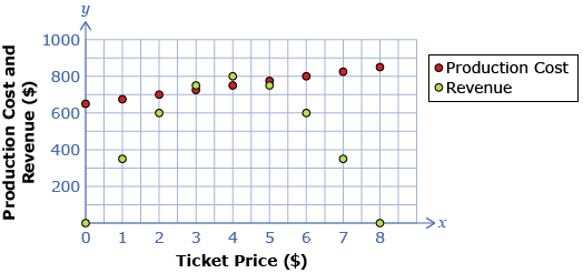
Mathematical models can be useful for making predictions. Consider the following scenario:
The treasurer of a drama club is putting together a budget for the club’s next production. She has determined the revenue the club can expect to generate for its next production as a function of ticket price. She has also determined the cost of the production, also as a function of ticket price. The following graph shows her predictions.
Data Source: PRINCIPLES OF MATHEMATICS 12 by Canavan-McGrath et al. Copyright Nelson Education Ltd. Reprinted with permission.
How could the treasurer determine the ticket price that would produce revenue greater than costs? One way would involve determining the equation of a function passing through the production cost data points and the equation of another function passing through the revenue data points.
In this lesson you will learn about different classes of polynomial functions—their characteristic shapes and algebraic forms.
Lesson Outcomes
At the end of this lesson, you will be able to
- sketch graphs that represent constant, linear, quadratic, and cubic functions
- relate characteristics of graphs of polynomial functions to the functions’ algebraic forms
Lesson Questions
You will investigate the following questions:
- How are the characteristics of the graph of a polynomial function related to the degree of the polynomial?
- How are the characteristics of the graph of a polynomial function related to the leading coefficient and constant term?
Assessment
Your assessment may be based on a combination of the following tasks:
- completion of the Lesson 1 Assignment (Download the Lesson 1 Assignment and save it in your course folder now.)
- course folder submissions from Try This and Share activities
- additions to Glossary Terms
- work under Project Connection
Self-Check activities are for your own use. You can compare your answers to suggested answers to see if you are on track. If you are having difficulty with concepts or calculations, contact your teacher.
Remember that these questions and activities provide you with the practice and feedback that you need to successfully complete this course. You should complete all the questions and place the answers in your course folder. Your teacher may wish to view the work to check on your progress and to see if you need help.
Time
Each lesson in Mathematics 30-2 EveryWare is designed to be completed in approximately two hours. You may find that you require more or less time to complete individual lessons. It is important that you progress at your own pace, based on your individual learning requirements.
This time estimation does not include time required to complete Going Beyond activities or the Module Project.
1.1. Launch
Module 4: Polynomials
Launch
Do you have the background knowledge and skills you need to complete this lesson successfully? Launch will help you find out.
Before beginning this lesson, you should be able to
- use function notation
- create tables of values, plot points, and graphs
- determine domain and range
- analyze linear functions and their graphs
- analyze quadratic functions and their graphs
- determine x- and y-intercepts
1.2. Are You Ready?
Module 4: Polynomials
Are You Ready?
Complete the following questions. If you experience difficulty and need help, visit Refresher or contact your teacher.
-
- Given the function f(x) = 3x − 6, find
- f(−1)
- f(0)
- f(3)
- x, when f(x) = 0
Answers - State the answers from question 1.a. as sets of ordered pairs. Answers
- Graph f(x) without technology. Answers
- State the domain and range for f(x). Answers
- State the x- and y-intercepts for f(x). Answers
- The slope y-intercept form of a line is y = mx + b, where m is the slope and b is the y-intercept. State the slope of f(x). Look at your answer to question e. for the y-intercept: Is it the same as the last number in the equation? Answer
- Given the function f(x) = 3x − 6, find
-
- Given the function g(x) = 2x2 − 4x − 6, find
- g(−2)
- g(0)
- g(4)
- x, when g(x) = 0
- State the answers from question 2.a. as sets of ordered pairs. Answers
- Graph g(x) without technology. Answers
- State the domain and range for g(x). Answers
- State the x- and y-intercepts for g(x). Answers
- The function g(x) is a quadratic function and can be written as g(x) = 2(x − 1)2 − 8.
- What is the vertex?
- What is the axis of symmetry?
- Describe whether the graph opens up or down.
- Is the graph wider or thinner than g(x) = x2? What number in the equation can be used to predict this?
- What is the minimum value?
- What are the domain and range?
Answers
- Given the function g(x) = 2x2 − 4x − 6, find
If you answered the Are You Ready? questions without difficulty, move to Discover.
If you found the Are You Ready? questions difficult, complete the Refresher.
1.3. Refresher
Module 4: Polynomials
Refresher

To be successful in creating graphs of functions, you need to know how to plot coordinates. If you feel you need a review of this, go to the Coordinates applet.
Instructions for use: Grab the point in the demonstration applet, and observe how the coordinates change as you move the point around. You may want to choose “show indicator lines” to remind yourself how the coordinates are determined.
For a review of domain and range, use the Domain and Range Compressor applet.
Instructions for use:
- Choose one of the graph types.
- To see the corresponding domain, drag the Domain Shadow slider all the way to the bottom. The corresponding domain shadow (i.e., the blue line along the x-axis) represents the domain of the function.
- To determine the corresponding range, drag the Range Shadow slider all the way to the left. The corresponding range shadow (i.e., the red line along the y-axis) represents the range of the function.
Screenshot reprinted with permission of ExploreLearning
Use the “Quadratics in Vertex Form—Activity A” gizmo to explore and investigate quadratic functions in f(x) = a(x − h)2 + k form. Click on the “Exploration Guide” and follow the directions to get the full use of this interactive multimedia piece.
Go back to the Are You Ready? section and try the questions again. If you are still having difficulty, contact your teacher.
1.4. Discover
Module 4: Polynomials
Discover
The drama club scenario presented in the Focus requires that you recognize shapes of scatter plots and relate them to polynomial functions. The following activity will help you recognize the shapes for constant, linear, quadratic, and cubic polynomial functions.
Try This 1
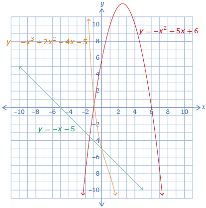
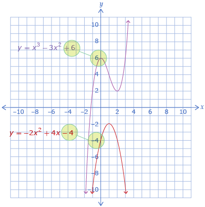
Open Polynomial Data Fitter. Your goal is to drag the blue points to make the line or the curve match the red points. If you can’t make the line or the curve match the red points, click one of the buttons (“Constant,” “Linear,” “Quadratic,” or “Cubic”) and try moving the blue points again.
Once you have matched the first set of red points, move the “Data Set” slider to select another set of red points to match.
Try This 1 gave you experience with the shapes of the graphs of constant, linear, quadratic, and cubic functions. You also saw the different equations for the graphs you were manipulating.
Share 1
With a partner or in a group, come to agreement on the typical shape, highest exponent, and sample equation for each type of function. You may want to organize your results in a table similar to the following. The entries for linear functions have been filled in for you.
Type of Function |
Highest Exponent |
Example Equation |
Example Shape |
Constant |
|
|
|
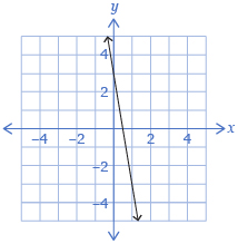
Linear |
1 |
f(x) = −5x + 3 |
|
Quadratic |
|
|
|
Cubic |
|
|
|
![]() If required, save a record of your discussion in your course folder.
If required, save a record of your discussion in your course folder.
1.5. Explore
Module 4: Polynomials
Explore
The shapes of the functions you experimented with in the Discover section are summarized in the following table.
Type of Function |
Highest Exponent |
Example Equation |
Example Shape |
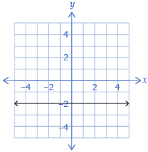
Constant |
0 |
f(x) = −2 |
|
Linear |
1 |
f(x) = −5x + 3 |
|
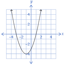
Quadratic |
2 |
f(x) = x2 + 2x − 3 |
|
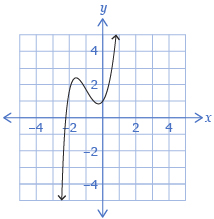
Cubic |
3 |
f(x) = 2x3 + 5x2 + 2x + 1 |
|

The functions you graphed in the Discover are all examples of polynomial functions.
A polynomial function contains only the operations of multiplication and addition with real numbers and variables. For example,
f(x) = 5x3 + 6x2 − 3x + 7
The function can also be written as
f(x) = 5(x)(x)(x) + 6(x)(x) + (−3)x + 7
From PRINCIPLES OF MATHEMATICS 12 by Canavan-McGrath et al. Copyright Nelson Education Ltd. Reprinted with permission.
In Discover you specified the highest exponent (on a variable). This is called the degree of the polynomial. In this module you will work with degree 0, 1, 2, and 3 polynomial functions.
Degree |
Name |
Example |
0 |
constant |
f(x) = 3.5 |
1 |
linear |
f(x) = 4x − 1 |
2 |
quadratic |
f(x) = 3x2 + 6x − 1 |
3 |
cubic |
f(x) = 5x3 − 4x2 + 7x + 3 |
Try This 1 introduced you to the general shapes and characteristics of polynomial functions. When describing a graph, it is often useful to consider the following characteristics:
- x-intercepts
- y-intercepts
- end behaviour
- domain
- range
- turning points
Most of these characteristics should be familiar to you; however, end behavior and turning points may be new.
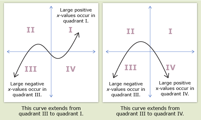
The end behaviour of a graph describes what happens as the x-values become very large positive or very large negative numbers. In this course, you will typically describe end behaviour by stating the quadrant the graph is in for large negative x-values and large postive x-values.
A turning point occurs when a graph changes from increasing to decreasing or from decreasing to increasing.
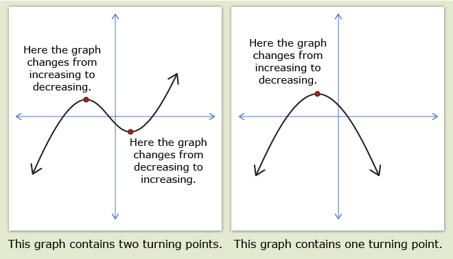
In the definition for turning point, describing a function that is decreasing means the curve is falling from left to right. Describing a function that is increasing means the curve is rising from left to right.
1.6. Explore 2
Module 4: Polynomials
Read “Explore the Math” on pages 274 and 275 of your textbook. In particular, pay attention to the definition for end behaviour. You should also read the definition for turning point on page 275. You will use end behaviour and turning points to help describe the characteristics of polynomial graphs.
Try This 2
Open Polynomial Function Explorer.
Your goal is to determine the following:
- number of possible x-intercepts
- number of possible y-intercepts
- end behaviour
- domain
- range
- number of possible turning points
Drag the blue points to explore the shapes of each type of function. (Click the buttons to change the function type.) It may be helpful to choose “Show x-intercepts” and “Show y-intercept.”
A table like the one that follows will help you organize your results.
Type of Function |
Constant |
Linear |
Quadratic |
Cubic |
Degree |
0 |
1 |
2 |
3 |
Example Function |
f(x) = a |
f(x) = ax + b |
f(x) = ax2 + bx + c |
f(x) = ax3 + bx2 + cx + d |
Possible Number of |
|
|
|
|
Possible Number of |
|
|
|
|
End Behaviour |
|
|
|
|
Domain |
|
|
|
|
Range |
|
|
|
|
Number of Possible Turning Points |
|
|
|
|
Adapted from PRINCIPLES OF MATHEMATICS 12 by Canavan-McGrath et al. Copyright Nelson Education Ltd. Reprinted with permission.
![]() Save your responses in your course folder.
Save your responses in your course folder.
1.7. Explore 3
Module 4: Polynomials
In Try This 1 you saw that the general shape of a graph can be predicted by the degree of the function. In Try This 2 you used the degree of a graph to predict some of the details of the graph.
A detailed summary of this information can be found in the table on page 276 of your textbook. Check to see how the following points relate to the table in the textbook.
- The degree of a function predicts its general shape: constant, linear, quadratic, or cubic.
- The number of x-intercepts is never greater than the degree.
- The number of y-intercepts is always one.
- For polynomials with an even degree, both ends of the graph will be above or both ends will be below the x-axis.
- For polynomials with an odd degree, one end of the graph will be above the x-axis and one end will be below the x-axis.
- Polynomials have a domain of {x|x ∈ R}.
- The range should be interpreted from the shape of the graph.
- The number of turning points is never greater than the degree minus 1.
Self-Check 1
Complete questions 1, 2, 3, and 4 on page 277 of your textbook. Answers
1.8. Explore 4
Module 4: Polynomials
In the first part of this lesson, you related the degree of polynomial functions to the shapes of the corresponding graphs. In the next part of this lesson, you will investigate the specific components of the equations that affect the corresponding graphs.
Try This 3
Use the End Behaviour Explorer to look for patterns in end behaviour and the y-intercepts. When the applet starts, a first degree (linear) function is shown. Change the “a” and “b” sliders, and pay attention to how the
- end behaviour of the function changes
- y-intercept changes (Be sure to check the “Show y-intercept” box.)
Repeat for degree 0, 2, and 3 polynomial functions.
- Which slider(s) affect the end behaviour of the graphs? Does the sign of this slider affect the end behaviour?
-
- Which slider(s) affect the y-intercept of the graphs?
- Record your observations in a table like the following.
Degree
Type of Function
End Behaviour
Starting Quadrant
Ending Quadrant
0
constant
1
linear
2
quadratic
3
cubic
![]() Save your responses in your course folder.
Save your responses in your course folder.
Share 2
With a partner or in a group, share your end behaviour observations from Try This 3. Once you come to agreement on end behaviour, discuss the following questions.
- Which parts of the polynomial can be used to predict end behaviour?
- Which parts of the polynomial can be used to predict the y-intercept?
![]() If required, place a summary of your discussion in your course folder.
If required, place a summary of your discussion in your course folder.
1.9. Explore 5
Module 4: Polynomials
In End Behaviour Explorer that you used to complete Try This 3, you may have found that only the leading coefficient, the a-value, affected the end behaviour. You should have also discovered that the end behaviour only changed if the sign of the leading coefficient changed.
The sign of the leading coefficient predicts end behaviour.
Cubic |
y = ax3 + bx2 + cx + d |
Quadratic |
y = ax2 + bx + c |
Linear |
y = ax + b |
Constant |
y = a |
Functions with a positive leading coefficient end in quadrant I. Functions with an even degree and positive leading coefficient begin in quadrant II, and functions with an odd degree and positive leading coefficient begin in quadrant III.
Functions with a negative leading coefficient end in quadrant IV. Functions with an even degree and negative leading coefficient begin in quadrant III, and functions with an odd degree and negative leading coefficient begin in quadrant II.
In Try This 3 you may have also found that the y-intercept has the same value as the constant term.
The value of the constant term predicts the y-intercept.
Cubic |
y = ax3 + bx2 + cx + d |
Quadratic |
y = ax2 + bx + c |
Linear |
y = ax + b |
Constant |
y = a |
The y-intercept is equal to the constant term for all polynomials.
1.10. Explore 6
Module 4: Polynomials
Read “In Summary” on page 286 of your textbook for further explanation of how the end behaviour and y-intercept can be determined from the equation of a function.
Then read the following textbook examples before moving on to Self-Check 2.
- “Example 1” on pages 279 to 281 shows how the characteristics of a polynomial function can be predicted from the equation of that function.
- “Example 2” on pages 282 and 283 shows how a function’s equation can be matched to a graph by exploring the characteristics predicted by the equation.
- “Example 3” on pages 284 and 285 shows how to sketch the graph of a function given some characteristics of that function.
Self-Check 2
Complete questions 1, 2, 3, 5, 6, 8, and 15 on pages 287 to 290 of your textbook. Answers
Add the following terms to your copy of Glossary Terms:
- degree
- end behaviour
- turning points
1.11. Connect
Module 4: Polynomials
Complete the Lesson 1 Assignment that you saved in your course folder at the beginning of the lesson. Show work to support your answers.
![]() Save your responses in your course folder.
Save your responses in your course folder.
Project Connection
Go to Module 4 Project: Graphic Design Using Polynomials and read the Project Overview to become familiar with what you will be doing and how you will be assessed. At this time, only read through the project. You will begin the project in Lesson 2.
1.12. Lesson 1 Summary
Module 4: Polynomials
Lesson 1 Summary
In this lesson you learned the relationships between polynomial degree and the following characteristics of the corresponding graph:
- x-intercept
- end behaviour
- domain
- range
- turning points
You also learned how the polynomial’s leading coefficient and constant term affect the end behaviour and the y-intercept, respectively.
In Lesson 2 you will learn how to determine lines of best fit for data points.