Lesson 2
| Site: | MoodleHUB.ca 🍁 |
| Course: | Math 30-2 SS |
| Book: | Lesson 2 |
| Printed by: | Guest user |
| Date: | Wednesday, 24 December 2025, 12:42 PM |
Description
Created by IMSreader
1. Lesson 2
Module 4: Polynomials
Lesson 2: Modelling Data with Lines of Best Fit
Focus

Brand X Pictures/Thinkstock
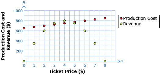
In Lesson 1 you learned about the drama club that determined the revenue it can expect to generate as a function of ticket price. The club also determined the cost of the production as a function of ticket price.
Data Source: PRINCIPLES OF MATHEMATICS 12 by Canavan-McGrath et al. Copyright Nelson Education Ltd. Reprinted with permission.
The following question was posed in Lesson 1: How could the ticket price be determined so that the club could expect revenue to be higher than costs? Finding the equation for a line that would pass through the production cost points would help create a useful model. The drama club would then be closer to finding a ticket price that would make a profit.
In this lesson you will learn how to determine the equation of a line of best fit using a process called regression.
Lesson Outcomes
At the end of this lesson, you will be able to
- use technology to determine the equation of a line of best fit
- use a regression equation to answer questions in a real-world context
Lesson Question
You will investigate the following question: How can a line of best fit be used to model problems?
Assessment
Your assessment may be based on a combination of the following tasks:
- completion of the Lesson 2 Assignment (Download the Lesson 2 Assignment and save it in your course folder now.)
- course folder submissions from Try This and Share activities
- additions to Glossary Terms
- work under Project Connection
1.1. Launch
Module 4: Polynomials
Launch
Do you have the background knowledge and skills you need to complete this lesson successfully? Launch will help you find out.
Before beginning this lesson, you should be able to
- determine the equation of a line from two points
- identify independent and dependent variables
1.2. Are You Ready?
Module 4: Polynomials
Are You Ready?
Complete the following questions. If you experience difficulty and need help, visit Refresher or contact your teacher.
- Determine the equation of a line that passes through the points (−2, 3) and (4, 6). State your answer in slope y-intercept form (y = mx + b). Answer
- Suppose you have collected some data on the time students spend studying (S) and their final grade (G) in their Mathematics 30-2 course.
- Which variable, S (time spent studying) or G (final grade), is the independent variable? How do you know?
- Which variable, S (time spent studying) or G (final grade), is the dependent variable? How do you know?
- If you were to plot your data, which variable would be plotted on the horizontal axis? Which data would be plotted on the vertical axis? How do you know?
Answers
If you answered the Are You Ready? questions without difficulty, move to Discover.
If you found the Are You Ready? questions difficult, complete the Refresher.
1.3. Refresher
Module 4: Polynomials
Refresher
Screenshot reprinted with permission of ExploreLearning
Use the “Slope-Intercept Form of a Line—Activity A” gizmo to explore and investigate lines in slope-intercept form. Click on the “Exploration Guide,” and follow the directions. Complete the five “Assessment Questions” within the gizmo. Then select “Check Your Answers” to ensure you understand this material.
Read the definition for independent and dependent variables found in the “Communication Tip” on the right-hand side of page 295 of your textbook. If you have not done so already, you should add these definitions to your copy of Glossary Terms.
Go back to the Are You Ready? section and try the questions again. If you are still having difficulty, contact your teacher.
1.4. Discover
Module 4: Polynomials
Discover
Comstock/Thinkstock
Read “Investigate the Math,” up to question A, on page 295 of your textbook. Notice how the relationship between variables can be used to make predictions.
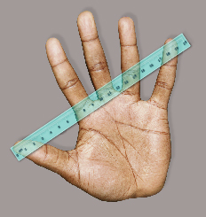
In the textbook, you read that Nathan wants to know if a person’s hand span is based on his or her height. To test this relationship, he recorded the heights and hand spans, both in centimetres, of 15 classmates.
Then he created the following scatter plot.
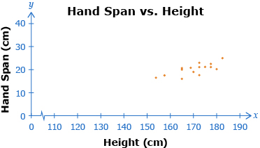
Data Source: PRINCIPLES OF MATHEMATICS 12 by Canavan-McGrath et al. Copyright Nelson Education Ltd. Reprinted with permission.
Try This 1
Use the Hand-Height Tool to create a line of best fit that best approximates the data acquired by Nathan. The line of best fit should approximate the trend in the data.
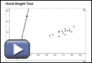
Record the equation of your line. What is the domain and range of your equation for the line of best fit?
![]() Save your responses in your course folder.
Save your responses in your course folder.
Share 1
With a partner or in a group, discuss answers for the following questions.
- What are your equations of the line of best fit? If they are different, explain why.
- What is the meaning of domain and range in the context of this problem? How do they relate to the domain and range you stated in Try This 1?
- How can a line of best fit be used to determine hand spans for people 140 cm and 160 cm tall?
![]() If required, place a summary of your discussion in your course folder.
If required, place a summary of your discussion in your course folder.
1.5. Explore
Module 4: Polynomials
Explore
You may have discovered in Share 1 that different people may determine different lines of best fit. Your lines were probably similar, but not exactly the same. The reason for this is that there is a trend to the data, but no exact line that goes through all data points.
algorithm: a specific set of steps for finding a solution to a problem
Mathematicians have created algorithms for creating the equations of lines that truly are “best” fit for the data. These algorithms minimize the difference between points in the scatter plot and points on the line. The resulting equation is called a regression equation and can be treated as a line of best fit. These algorithms have been implemented in spreadsheet programs and graphing calculators.
Once you have a regression equation, it can be used to answer questions for the problem.
Refer to the statistics section of your calculator’s manual to determine how to create regression equations. You will need to find a method to do the following:
- Clear all lists so you are sure that you start with no data in the lists.
- Enter lists of data.
- Create a linear regression equation. (Look for “y = ax + b.”)
If you have difficulty with any of these steps, contact your teacher for assistance.
Try This 2
Enter the data from the table on page 295 of your textbook into your calculator; the data is also shown in the Discover. Enter the height values as the first list and the hand span values as the second. If you have difficulty with any of the steps in determining a linear regression equation, consult your calculator manual or contact your teacher.
-
- Now perform the steps to find the linear regression equation.

- How does this regression equation compare to the equation of the line of best fit you determined in Try This 1?
- Now perform the steps to find the linear regression equation.
- Use your regression equation to predict the hand span for a person who is
- 140 cm tall
- 160 cm tall
![]() Save your responses in your course folder.
Save your responses in your course folder.
1.6. Explore 2
Module 4: Polynomials
In Try This 2, you used your calculator to determine a linear regression. If you graphed the regression equation along with the data points, it would have looked like the following.
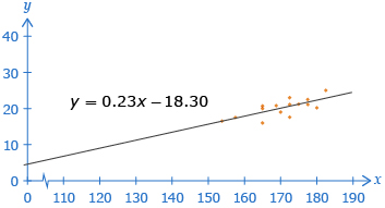
A regression equation can be treated like a line of best fit.
A height of 160 cm was within the domain of the given data. Using a regression equation for an x-value in the domain of the data is called interpolation.
A height of 140 cm was not within the domain of the given data. Using a regression equation for an x-value not in the domain of the data is called extrapolation.
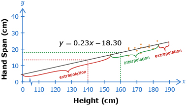
Predicting the hand span of a person who is 140 cm is an extrapolation, because 140 cm is outside the data set. Predicting the hand span of a person who is 160 cm is an interpolation, because
160 cm is within the data set.
Read “Example 1” on pages 296 to 299 of your textbook. In this example, linear model is referring to a linear regression equation. Pay particular attention to the following differences in Carmen’s and Sandra’s solutions:
- values for x (representing year) used to create the equations
- method used for estimating a possible world-record distance for 2006
Self-Check 1
Complete questions 1, 2, and 4 on pages 301 and 302 of your textbook. Answers
1.7. Explore 3
Module 4: Polynomials
Both linear regression equations and lines of best fit can be used to make predictions based on a set of data. In Try This 3, you will explore how multiple sets of data can be used to solve a problem.
Try This 3

Stockbyte/Thinkstock
Jean and Mohammad were discussing health issues and what blood pressure tells you. Jean said that systolic blood pressure is affected by age, and Mohammad said he believed it was related more closely to weight. They obtained the following data for ten patients.
Age |
Weight (lb) |
Systolic Pressure (mmHg) |
52 |
173 |
130 |
59 |
184 |
143 |
68 |
194 |
153 |
73 |
210 |
162 |
65 |
196 |
154 |
74 |
220 |
168 |
61 |
188 |
150 |
66 |
207 |
159 |
46 |
167 |
130 |
72 |
220 |
166 |
You want to test both Jean’s and Mohammad’s hypotheses.
-
- Consider Jean’s hypothesis. Which variable is dependent, and which is independent? Explain your reasoning.

- Create a scatter plot for Jean’s hypothesis.
- Consider Jean’s hypothesis. Which variable is dependent, and which is independent? Explain your reasoning.
-
- State which variable is independent and which is dependent for Mohammad’s hypothesis.
- Create a scatter plot for Mohammad’s hypothesis.
- Explain whose hypothesis is more likely to be correct by referring to the scatter plots.
-
- Explain why it is reasonable to use a line of best fit for both graphs. For what kind of scatter plot is it unreasonable to use a line of best fit?
- Determine the equation of a line of best fit for both scatter plots.
- What would be the expected systolic blood pressure for an 80 year old?
- What would be the expected blood pressure for a person weighing 300 lb?
![]() Save your responses in your course folder.
Save your responses in your course folder.
Share 2
With a partner or in a group, discuss answers for the following questions.
- Did you agree about who had the correct hypothesis? If not, explain why.
- Were your equations of the lines of best fit the same? Explain why or why not.
- What would be an appropriate domain and range for each of your lines of best fit?
![]() If required, place a summary of your discussion in your course folder.
If required, place a summary of your discussion in your course folder.
1.8. Explore 4
Module 4: Polynomials
In Try This 3, you used lines of best fit to compare different sets of data. In that activity, you may have found that a linear regression was reasonable for both graphs because the data tended to follow a straight line. If the data does not follow a straight line, it is not reasonable to use a line of best fit or linear regression.
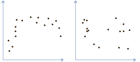
Neither a line of best fit nor a linear regression should be used with these sets of data because neither graph follows a straight-line pattern.
Self-Check 2
- Ahmed is planning a vacation. He would like to know how much money he would need for spending money. He asked his friends who have taken vacations how much they spent on their holidays. He then created a scatter plot of this data and found a line of best fit.
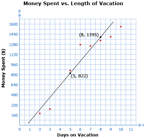
- Using the two points provided on the line of best fit, find the equation of the line in slope y-intercept form. Make sure to round the slope and the y-intercept to the nearest whole number. Answer
- State an appropriate domain and range for this problem. Answer
- Using your model (i.e., the equation of the line of best fit), how much could Ahmed expect to spend if he is on vacation for four days? Answer
- Using your model, if Ahmed has $1700 set aside, for how many days would he have spending money? Answer
![]()
- Complete questions 3, 5, and 6 on pages 301 and 302 of your textbook. Answer
Add the following terms to your copy of Glossary Terms:
- regression equation
- interpolation
- extrapolation
1.9. Connect
Module 4: Polynomials
Complete the Lesson 2 Assignment that you saved in your course folder at the beginning of the lesson. Show work to support your answers.
![]() Save your responses to your course folder.
Save your responses to your course folder.
Project Connection
You are now ready to apply your understanding of the different types of polynomials to their existence in in your environment. Go to the Module 4 Project: Graphic Design Using Polynomials. Complete Part 1.
1.10. Lesson 2 Summary
Module 4: Polynomials
Lesson 2 Summary
In this lesson you learned how to create regression equations for data that has a linear trend. You used these equations to make conclusions using interpolation and extrapolation. There are many applications of linear equations in fields such as business, advertising, and science. Reflect on what you have learned and whether or not you have experienced the use of linear equations to make predictions or inferences before.
In Lesson 3 you will be introduced to data that does not have a linear trend, and you will explore the various ways of dealing with non-linear data.