Lesson 3
| Site: | MoodleHUB.ca 🍁 |
| Course: | Math 30-2 SS |
| Book: | Lesson 3 |
| Printed by: | Guest user |
| Date: | Wednesday, 24 December 2025, 12:44 PM |
Description
Created by IMSreader
1. Lesson 3
Module 4: Polynomials
Lesson 3: Modelling Data with a Curve of Best Fit
Focus
In Lesson 2 you were introduced to using linear regression to draw conclusions about data that exhibits a linear trend. What about data that does not have a linear trend? For example, what about the revenue data from the drama scenario introduced in Lesson 1?
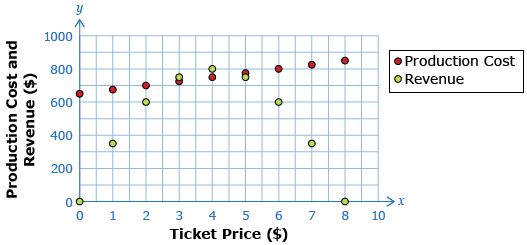
Data Source: PRINCIPLES OF MATHEMATICS 12 by Canavan-McGrath et al. Copyright Nelson Education Ltd. Reprinted with permission.
In this lesson you will learn about quadratic and cubic regressions and use those equations to model real-world problems.
Lesson Outcomes
At the end of this lesson you will be able to
- use technology to determine quadratic and cubic regression equations
- use a regression equation to answer questions in a real-world context
Lesson Question
You will investigate the following question: How can a curve of best fit be used to model problems?
Assessment
Your assessment may be based on a combination of the following tasks:
- completion of the Lesson 3 Assignment (Download the Lesson 3 Assignment and save it in your course folder now.)
- course folder submissions from Try This and Share activities
- work under Project Connection
1.1. Launch
Module 4: Polynomials
Launch
Do you have the background knowledge and skills you need to complete this lesson successfully? Launch will help you find out.
Before beginning this lesson, you should be able to
- solve quadratic equations algebraically
- solve quadratic equations graphically
- determine characteristics of the graph of a quadratic function from its equation
1.2. Are You Ready?
Module 4: Polynomials
Are You Ready?
Complete the following questions. If you experience difficulty and need help, visit Refresher or contact your teacher.
Solving means “find the value(s) of x that makes an equation true.”
- Solve the following quadratic equations by graphing.
- Solve by graphing.

- Solve by using the quadratic formula.
- Given the following quadratic function, find the equation in vertex form y = a(x − p)2 + q.
Answer
If you answered the Are You Ready? questions without difficulty, move to Discover.
If you found the Are You Ready? questions difficult, complete Refresher.
1.3. Refresher
Module 4: Polynomials
Refresher
Use Solving Quadratic Equations: Using Graphs for help with solving by graphing. It is suggested you skip the introduction and go directly to the tutorial section by selecting the chalkboard icon near the top of the window.

Source: Khan Academy
(![]() BY-NC-SA 3.0)
BY-NC-SA 3.0)
For help with solving quadratic equations using the quadratic formula, watch the video titled “Applying the Quadratic Formula.”
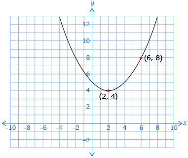
For help with finding the equation of a quadratic function when you are given the vertex and at least one other point on the curve, go to Finding the Equation of a Quadratic Function.
Go back to the Are You Ready? section and try the questions again. If you are still having difficulty, contact your teacher.
1.4. Discover
Module 4: Polynomials
Discover
Read “Investigate the Math,” up to question A, on page 307 of your textbook.
Try This 1
Use the Ball Bouncing Tool applet to create a curve of best fit. Drag the blue points so that the resulting curve matches the trend of the data.
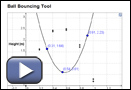
Use the coordinates of the blue points to determine the equation of your curve. ![]()
- What type of function is your curve of best fit?
- How can the curve of best fit be used to determine how long the ball is in the air?
![]() Save your responses in your course folder.
Save your responses in your course folder.
Share 1
With a partner or in a group, come to agreement on the answers to the Try This 1 questions. Then discuss the following: Why is linear regression inappropriate for this problem?
![]() If required, save a record of your discussion in your course folder.
If required, save a record of your discussion in your course folder.
1.5. Explore
Module 4: Polynomials
Explore
What you may have concluded in Share 1 is that linear regression is not appropriate for the bouncing ball data for two reasons:
- Graphical: The data is clearly not linear as the y-coordinates increase and then decrease.
- Contextual: After the ball goes up, it must come down—a process that can’t be modelled with a straight line.
The curve you created in Try This 1 is quadratic. As with linear data, spreadsheets and graphing calculators can perform quadratic regressions.
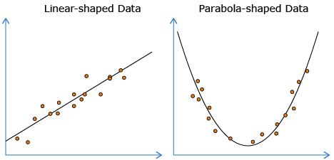
Linear regressions can be used with linear-shaped data. Quadratic regressions can be used with parabola-shaped (U) data.
When using a graphing calculator, the quadratic regression command is usually found in the same menu as linear regression.
The quadratic regression equation for the bouncing ball data calculated using a graphing calculator is y = −9.79x2 + 10.01x, where x is time in seconds and y is height in metres.
Notice that function matches trend of the data.
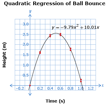
A regression equation that approximates the data can be used to determine how long the ball is in the air. Since the ball starts on the ground at time zero, the time it lands for the second bounce will be equal to the time it is in the air.
The ground is at height y = 0, so substituting 0 into the equation results in the following equation to be solved:
0 = −9.79x2 + 10.01x
The right side of this equation can factored:
![]()
By the zero product factor property:
or
Sometimes a quadratic equation cannot be solved by factoring. In these cases, the quadratic formula can be used:
The first answer, 0 s, corresponds to the first bounce. The second answer, 1.02 s, corresponds to the second bounce and the length of time that the ball is in the air.
Read “Example 1” on pages 308 to 310 of your textbook. Pay attention to the similarities between how a quadratic regression is used in this example and how linear regressions were used in the last lesson.
Self-Check 1
Complete questions 1, 3, 6, and 7 on pages 313 to 315 of your textbook. Answers
1.6. Explore 2
Module 4: Polynomials
If the points on a scatter plot seem to follow a trend or pattern, it is important to establish what shape the trend is taking to decide what type of regression is appropriate.
Try This 2
For questions 1 and 2, provide the following information:
- Predict what shape or trend the data is going to take before plotting it.
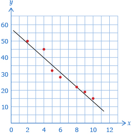
- Plot the data and find the equation of the regression line or curve.
- Sketch the line or curve of best fit on your scatter plot.
- State what type of data is modelled.
- (2, 50)
(4, 45)
(5, 32)
(6, 28)
(8, 22)
(9, 19)
(10, 15) -
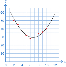
(2, 50)
(3, 45)
(5, 32)
(6, 28)
(8, 34)
(9, 36)
(10, 40)
![]() Save your responses in your course folder.
Save your responses in your course folder.
1.7. Explore 3
Module 4: Polynomials
In Try This 2, you should have discovered that the data in part a. was linear. You may have noticed that as the x-values increased, the y-values decreased.
For part b., you should have found that the data was quadratic. You may have been able to predict this by noticing that as the x-values increased, the y-values decreased initially and then increased in the later data. This created a parabolic shape.
Data can model other patterns as well. The last type of regression you will study in this module is the cubic regression. (There are other forms of regression, some of which you will see in other modules.)
1.8. Explore 4
Module 4: Polynomials
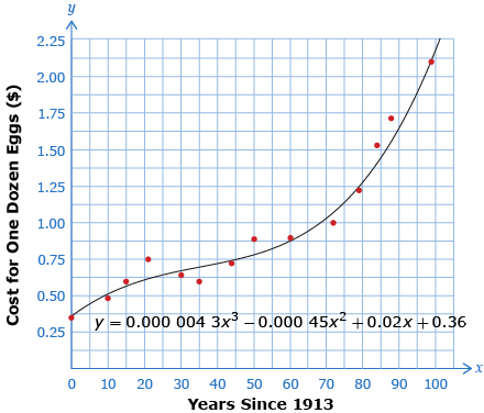
Consider the following data. The table shows the cost of one dozen eggs from 1913 to present day.
| Year Since 1913 | 0 | 10 | 15 | 22 | 30 | 35 | 44 | 50 | 60 | 72 | 79 | 84 | 88 | 99 |
| Cost of One Dozen Eggs ($) | 0.35 | 0.48 | 0.60 | 0.75 | 0.64 | 0.60 | 0.72 | 0.88 | 0.90 | 1.00 | 1.22 | 1.54 | 1.70 | 2.10 |

iStockphoto/Thinkstock
Draw a scatter plot of the data. Then compare your scatter plot with the following.
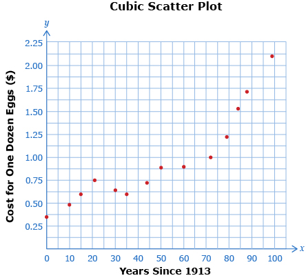
What do you notice? Is the data linear? quadratic? neither?
The data is neither linear nor quadratic and would best be modelled by a cubic function.
Use your graphing calculator to find the cubic regression equation (much like you have found the linear regression equations and quadratic regression equations).
The equation from your calculator (after some rounding) should be
y = 0.000 004 3x3 − 0.000 45x2 + 0.02x + 0.36
Plotting the cubic curve of best fit yields the following graph:
Self-Check 2
1.9. Explore 5
Module 4: Polynomials
You need to be careful when modelling data using a regression. Sometimes the regression equation will tell you things that don’t make sense. Try This 3 explores this idea.
Try This 3
The number of births to women of a particular demographic in the United States is listed in the following table.
Year |
Years Since 1970 |
Births (thousands) |
1970 |
0 |
11.752 |
1980 |
10 |
10.169 |
1986 |
16 |
10.176 |
1990 |
20 |
11.657 |
1991 |
21 |
12.014 |
1992 |
22 |
12.220 |
1993 |
23 |
12.554 |
1994 |
24 |
12.901 |
1995 |
25 |
12.242 |
1996 |
26 |
11.146 |
1997 |
27 |
10.121 |
1998 |
28 |
9.462 |
1999 |
29 |
9.054 |
2000 |
30 |
8.519 |
2001 |
31 |
7.781 |
2002 |
32 |
7.315 |
2003 |
33 |
6.661 |
-
- Predict the shape of the scatter plot by looking at the data. Which regression model that you have learned so far would best model this data?
- Plot the data using a graphing calculator.

- Does the scatter plot cause you to change your mind about the type of regression that would best fit this data?
-
- Use your calculator to determine a regression equation for the data. Make sure to round your values to four decimal places.
- Graph the regression equation on the same graph as your scatter plot. Does the graph of the equation appear to match the data?
- Use your calculator to determine a regression equation for the data. Make sure to round your values to four decimal places.
-
- Estimate the number of births in 1975.
- Estimate the number of births in 2010.
- Describe a problem with the prediction for 2010.
- Estimate the number of births in 1975.
- Use the graph of your regression equation to predict a year when 3000 births will occur.
![]() Save your responses in your course folder.
Save your responses in your course folder.
1.10. Explore 6
Module 4: Polynomials
In Try This 3, you saw that the cubic regression equation sometimes predicts unrealistic values and that you need to be careful when using a model to make predictions. Typically, interpolation (predicting a value within the data) is much more reliable than extrapolation (predicting a value outside the data).
Just as in the egg example, you may have noticed that solving the equation 3 = −0.0014x3 + 0.064x2 − 0.6399x + 11.7298 can be done by graphing both sides of the equation and finding the intersection.
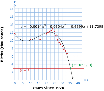
The graphs of y = −0.0014x3 + 0.064x2 − 0.6399x + 11.7298 and
y = 3 intersect at (35.1896, 3). Therefore, 35.1896 is a solution to the equation 3 = −0.0014x3 + 0.064x2 − 0.6399x + 11.7298.
Read “Example 2” on pages 310 to 312 of your textbook to see how a cubic regression can be used to model data. Pay attention to how Brad determines the year gas prices were 56.0¢/L.
Self-Check 3
Complete questions 2, 5, and 9 on pages 313 to 315 of your textbook. Answers
1.11. Connect
Module 4: Polynomials
Complete the Lesson 3 Assignment that you saved in your course folder at the beginning of the lesson. Show work to support your answers.
![]() Save your responses in your course folder.
Save your responses in your course folder.
Project Connection
You are now ready to complete your project. Go to the Module 4 Project: Graphic Design Using Polynomials. You will complete Part 2, which deals with regression curves that meet specific parameter requirements. Submit your project to your teacher when it is complete.
1.12. Lesson 3 Summary
Module 4: Polynomials
Lesson 3 Summary

Jupiterimages/Photos.com/Thinkstock
In this lesson you learned how to create regression equations for data that has quadratic or cubic trends. You used these equations to make and solve contextual problems using interpolation and extrapolation.
The skills of interpolation and extrapolation are important tools that you may use later in life. Imagine that you are hired to provide catering for a group of 100 people. You are, however, informed at the last minute that you will be only be catering for 74 people. You will be able to make the appropriate changes.
These skills also come in handy when making predictions and analyzing information in job situations.
You will even see the use of these skills when predicting the orbits of planets and comets, times of flights for objects, and price increases of certain items.
Regression equations and interpolation, as well as extrapolation, can often be seen in the news when reports of housing prices, inflation, and cost of living are calculated. Keep this in mind as you prepare for your final research project for this course.