Lesson 7
| Site: | MoodleHUB.ca 🍁 |
| Course: | Math 30-2 SS |
| Book: | Lesson 7 |
| Printed by: | Guest user |
| Date: | Wednesday, 24 December 2025, 4:25 AM |
Description
Created by IMSreader
1. Lesson 7
Module 7: Exponents and Logarithms
Lesson 7: Modelling Data Using Exponential and Logarithmic Regressions
Focus
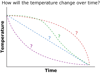
Imagine your favourite warm drink, perhaps tea or hot chocolate. The drink is nice and hot when it’s first made; however, the drink will cool off as it sits. Clearly the temperature is decreasing, but what would a graph of temperature versus time look like? Would it be a straight line? A curve? One way to determine what this graph looks like is to collect data and perform a regression.
In this lesson you will learn about exponential and logarithmic regression, and you will use those equations to model real-world problems.
Lesson Outcomes
At the end of this lesson, you will be able to
- use technology to determine exponential and logarithmic regression equations
- use a regression equation to answer questions in a real-world context
Lesson Question
You will investigate the following question: How can an exponential or logarithmic model be used to solve problems?
Assessment
Your assessment may be based on a combination of the following tasks:
- completion of the Lesson 7 Assignment (Download the Lesson 7 Assignment and save it in your course folder now.)
- course folder submissions from Try This activities
- additions to Glossary Terms
- work under Project Connection
1.1. Launch
Module 7: Exponents and Logarithms
Launch
Do you have the background knowledge and skills you need to complete this lesson successfully? Launch will help you find out.
Before beginning this lesson, you should be able to
- use technology to determine the equation of a line of best fit
- use technology to determine the equation of a curve of best fit (quadratic and polynomial)
- use a regression equation to answer questions in a real-world context
1.2. Are You Ready?
Module 7: Exponents and Logarithms
Are You Ready?
Complete these questions. If you experience difficulty and need help, visit Refresher or contact your teacher.
- Logos-to-Go is a company that travels around Alberta supplying teams with hoodies featuring unique logos. The company needs to buy the plain hoodies in bulk to help save money. However, Logos-to-Go does not want to be left with too much stock at the end of each season. The price per hoodie is related to the size of the bulk order. Seven of Logos-to-Go past orders are listed in the following table:
Number of Hoodies Cost per Hoodie ($) 400 22 600 19 250 27 720 18 330 25 820 16 500 21 - Use technology to create a scatter plot and determine an equation for the linear regression function that models this data. Answer
- What do the slope and y-intercept in the regression equation represent in this question? Answer
- Use the linear regression function model to extrapolate and find the size of order needed to achieve a cost of $15 per hoodie. Answer
- Chuck is a pitcher for his local slow-pitch team. The height of the ball after being pitched is listed in the following table:
Time (s) 0 0.33 0.67 1.0 1.3 Height (m) 1 2.8 3.5 3.1 1.6
If you answered the Are You Ready? questions without difficulty, move to Discover.
If you found the Are You Ready? questions difficult, complete Refresher.
1.3. Refresher
Module 7: Exponents and Logarithms
Refresher
Review Try This 2 of Math 30-2: Module 4: Lesson 2 to review creating a graph and equation based on a linear set of data and extracting information from the graph and equation.
Khan Academy
(![]() BY-NC-SA 3.0)
BY-NC-SA 3.0)
Open “Linear Regressions” to see how to make predictions using a linear model.
Review Try This 1 of Math 30-2: Module 4: Lesson 3 to review creating a graph and equation based on a set of quadratic data and extracting information from the graph and equation.
Khan Academy
(![]() BY-NC-SA 3.0)
BY-NC-SA 3.0)
Go to “Quadratic Regressions” to see how to make predictions using a quadratic model.
Go back to the Are you Ready? section and try the questions again. If you are still having difficulty, contact your teacher.
1.4. Discover
Module 7: Exponents and Logarithms
Discover
Try This 1

George Doyle/Stockbyte/Thinkstock
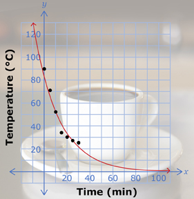
Each morning a teacher reads the newspaper. He does this with a nice fresh cup of coffee. Many mornings, however, he becomes so focused on his newspaper that the coffee becomes cold and unpleasant to drink.
The following data shows the temperature of the cup of coffee as it sits cooling.
| Time (in min) | Temperature (°C) |
| 0 | 90 |
| 5 | 71 |
| 10 | 52 |
| 15 | 34 |
| 20 | 30 |
| 25 | 27 |
| 30 | 25 |
- Use your graphing calculator to plot the data.

- Is the temperature increasing or decreasing?
- What is the shape of your scatter plot? What kind of model do you expect to use with this data?
- Use your calculator to find a regression equation.
- Graph the regression equation on the same graph as the scatter plot.
- What is an appropriate domain and range for this situation?
1.5. Explore
Module 7: Exponents and Logarithms
Explore
In Try This 1, you may have discovered that the model that would best fit the cooling cup of coffee is the exponential regression equation y = 82.63(0.956)x. This is the form of exponential equation you saw in Lesson 1 (y = abx, b > 0, b ≠ 1). The data points lie close to this function; therefore, it is a good model for the data.
Adapted from Stockbyte/Thinkstock
Read “Example 1” on pages 371 to 373 of your textbook to see how an exponential regression can be used to make predictions using interpolation and extrapolation. In this problem, time is inputted as 10-year increments instead of using the years listed in the table. Typically, when years (such as 1871 or 1992) are used when performing a regression, the resulting equation is very sensitive to rounding. To avoid this, the number of years past a time is often used for regressions. In this example, 10-year increments are used.
Read and note the section titled “Key Idea” on the bottom of page 376. This provides a summary of exponential regression.
Self-Check 1
1.6. Explore 2
Module 7: Exponents and Logarithms
So far in this lesson, you have looked at exponential regressions. Next, you will focus on logarithmic regressions.
Try This 2
iStockphoto/Thinkstock
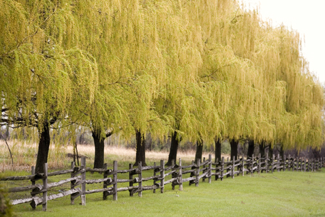
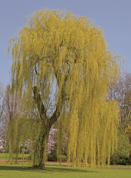
The Iverson family ordered some trees from the provincial shelterbelt program to plant on their acreage.
The following data shows the average growth rate of 20 weeping willow trees after planting. At the time of planting, all the trees were 2 ft in height and were 1 y old.
| Age of Trees (Years) |
Average Height (Feet) |
| 1 | 2 |
| 2 | 4.8 |
| 3 | 6.4 |
| 4 | 9.5 |
| 5 | 13 |
| 6 | 15.2 |
| 7 | 16.6 |
| 8 | 17.8 |
| 9 | 18.5 |
| 10 | 19 |
| 11 | 19.4 |
| 12 | 19.6 |
- Use your graphing calculator to plot the data.
- Is the average height increasing or decreasing?
- What is the shape of your scatter plot? What kind of model do you expect to use with this data?
- What is an appropriate domain and range in this situation?
![]() Save your responses in your course folder.
Save your responses in your course folder.
1.7. Explore 3
Module 7: Exponents and Logarithms
iStockphoto/Thinkstock
If you identified that the weeping willow tree growth looked like a logarithmic function, you are correct. The growth is also an increasing function, as the trees are getting taller as time passes.
Most graphing calculators provide the logarithmic regression equation in the form y = a + b ln x. The abbreviation ln is referring to loge and is usually called a natural logarithm. The number e is an irrational number, like π, and is approximately 2.718. Natural logarithms are important in advanced mathematics, so most regression programs use it instead of log10.
Determine a logarithmic regression equation for the data in Try This 2.
If you are unsure how to calculate a logarithmic regression, see your calculator manual or contact your teacher.
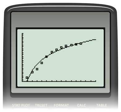
The logarithmic regression for the tree data is y = −0.068 + 8.136 (ln x). Make sure that you are able to do this on your calculator. Graph this function on the same grid as the scatter plot.
The screen on your graphing calculator should look similar to the following:
Self-Check 2
Using your logarithmic regression model from the weeping willow tree example, answer the following questions.
- Interpolate: What was the average height of the trees at 2.5 y of age (to the nearest tenth of a foot)? Answer
- Extrapolate: What is the predicted average height of the trees at 20 y of age (to the nearest tenth of a foot)? Is this prediction realistic? Answer
- According to your model, if the average height of the trees is 17 ft, what is the age of the trees to the nearest tenth of a year? Answer
- Complete question 8 on page 470 of your textbook. Answer
1.8. Explore 4
Module 7: Exponents and Logarithms
A logarithmic regression equation
- can be of the form y = a + b ln x
- has end behaviour that extends from quadrant IV to quadrant I (increasing) or quadrant I to quadrant IV (decreasing)
Read “Example 2” on pages 463 to 465 of your textbook to see how a logarithmic regression can be performed and used to solve problems. Also, read and note the section titled “Key Idea” on the top of page 466, which summarizes logarithmic regressions.
You have now used exponential and logarithmic regressions to model data. In Try This 3, you will use your understanding of the characteristics of both these types of equations to match equations to their graphs.
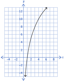
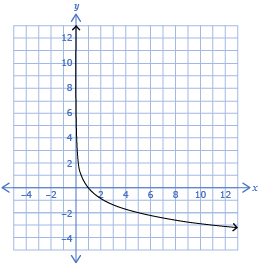
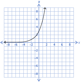
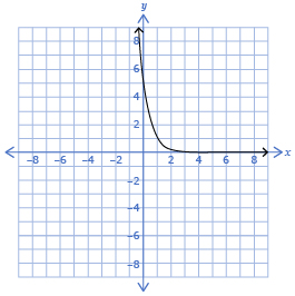
Try This 3
Open Matching Exponential and Logarithmic Equations and Graphs, and match each equation with the correct corresponding graph.
1.9. Explore 5
Module 7: Exponents and Logarithms
In Try This 3, you reviewed the characteristics of exponential and logarithmic equations and their graphs. These characteristics are summarized in the following table. You used these characteristics to match equations to their graphs.
| Form | y-intercepts | x-intercepts | Graph Increases | Graph Decreases | |
| Exponential Functions | y = a(b)x | one y-intercept that equals the a-value | no x-intercepts | If b > 1, the graph is increasing. | If 0 < b < 1, the graph is decreasing. |
| Logarithmic Functions | y = a + b ln x | no y-intercepts | one x-intercept | If 0 > b > 1, the graph is increasing. | If 0 > b < 1, the graph is decreasing. |
Self-Check 3
- Complete question 1.a. on page 466 of the textbook. Answer
- Match the given functions with the appropriate graphs. Provide an explanation for your choice.
i. y = 3(2)x ii. y = 5 log2 (x) iii. 
iv. y = −2 log5 (x)
Answer
Add the following terms to your copy of Glossary Terms:
- natural logarithm
- logarithmic regression
1.10. Connect
Module 7: Exponents and Logarithms
Connect
Lesson 7 Assignment
Complete the Lesson 7 Assignment that you saved in your course folder at the beginning of this lesson. Show work to support your answers.
![]() Save your responses in your course folder.
Save your responses in your course folder.
Project Connection
You are now ready to complete your project. Go to Part 3: Research Movie Revenues of the Module 7 Project: At the Movies. Complete Activity 2: Research Your Own Movie and the Conclusion. Submit your project to your teacher when it is complete.
1.11. Lesson 7 Summary
Module 7: Exponents and Logarithms
Lesson 7 Summary
In this lesson you looked at data that modelled either exponential or logarithmic behaviour. You were introduced to both exponential and logarithmic regression. The general formula for exponential functions, y = a(b)x, was applied to the exponential data, and the formula y = a + b ln x was used when investigating and using logarithmic regression.