Lesson 3
Completion requirements
Created by IMSreader
1. Lesson 3
1.11. Lesson 3 Summary
Module 2: Radical Functions
Lesson 3 Summary
In this lesson you explored solving radical equations graphically. The solutions, or roots, of a radical equation are equivalent to the x-intercepts of the corresponding radical function. Two graphical methods were discussed.
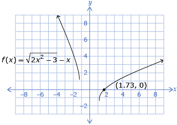
Using a single function:
- Rearrange the equation so that one side is equal to zero, and then graph the function. The solution is found by determining the value of the x-intercept(s).
- The solution of the equation
 is x ≈ 1.73.
- The solution for the equation is 1.73.
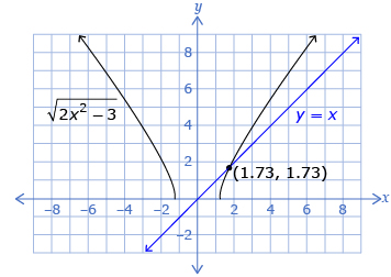
Using a system of two functions:
- Graph each side of the equation as two separate functions. The solution is determined by the value of x at the point(s) of intersection.
- The solution of the equation
 is x ≈ 1.73.
Radical equations that are used in various contexts, such as accelerated motion, can be solved using a graphical method.