Lesson 8
1. Lesson 8
1.12. Lesson 8 Summary
Module 4: Quadratic Equations and Inequalities
Lesson 8 Summary

© morganimation/12959959/Fotolia
In this lesson you investigated the following questions:
- What principle is common to all strategies for solving quadratic inequalities?
- How can you tell when a problem can be modelled by a quadratic inequality in one variable?
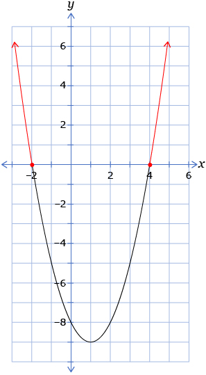
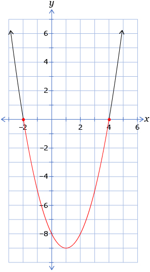
In this lesson you learned that quadratic inequalities in one variable can be solved in a number of different ways. Whether you solve quadratic inequalities in one variable graphically or algebraically, there is one principle that is common to them all. A quadratic inequality can be greater than 0 or less than 0, which means that the y-values are either positive or negative.
Therefore, regardless of the method you choose, you must determine solutions based on whether the y-coordinates in the solution are positive or negative. The following table summarizes how you determine the solution intervals based on signs.
| Strategy for Solving | How to Determine the Solution Interval(s) |
| Graphing | Look above the x-axis if f(x) > 0 or f(x) ≥ 0.
Look below the x-axis if f(x) < 0 or f(x) ≤ 0.
|
| Roots and Test Points | Use a test point from each interval to determine if the interval will yield positive or negative values of the function.
|
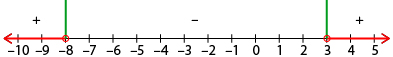
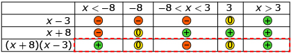
| Sign Analysis | Consider the signs of the factors at each interval. Select the solution interval(s) based on the signs of the product of the factors.
|
| Case Analysis | Consider what the signs of the factors could be in order to satisfy the inequality based on the following four possible cases:
Then graph each possible case to determine the solution intervals. |
You also modelled problems with quadratic inequalities in one variable. There are two conditions that are common to such problems. The first is that the situation can be represented by a quadratic function. The second is that the problem asks about points on the function that are greater than or less than a reference point.