Lesson 3
1. Lesson 3
1.1. Discover
Module 4: Statistical Reasoning
Discover
Have you ever noticed how graphs of data can have different shapes? For instance, the frequency distributions for Mr. Kong’s Block 1 and Block 4 quiz marks have different shapes.
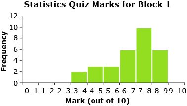
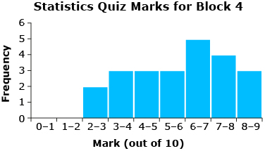
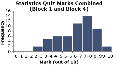
Each one of the graphs for the quiz marks has only one peak.
Take a look at the shapes of the following graphs and consider this question: What information can the shape of the graph provide about the data? Think about what the number of peaks tells you about the data.
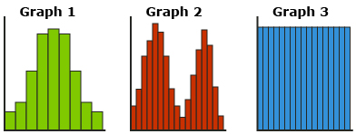
Here is some information you might determine based on the shape of the graph.
- One peak means there is one mode (i.e., unimodal, one number that occurs most frequently). The data looks like it is symmetrical about the peak (half the data is above the peak and half the data is below the peak).
- Two peaks means there are two modes (i.e., bimodal, two numbers that occur most frequently).
- No peaks means there are no modes (i.e., all the numbers occur with the same frequency).
Frequency distributions (i.e., graphs) help to visualize and summarize data. Graphs are also useful to help determine if data approximates a normal distribution.
normal distribution: data that produces a graph that is unimodal (has one mode) and symmetrical about the mean
The mean, median, and mode of a normal distribution are equal (or close) and fall at the line of symmetry.
— From CANAVAN-MCGRATH ET AL. Principles of Mathematics 11, © 2012 Nelson Education Limited. Reproduced by permission.
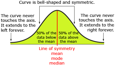
normal curve (bell curve): symmetrical curve with a central peak at the mean of the data
A normal distribution of data has a graph that is shaped like a bell. There is one mode (i.e., peak) and the data is symmetrically distributed about the mean. In other words, there is the same amount of data above the mean as below the mean. Most values are near the middle or mean of the graph with very few values near the upper and lower extremes of the graph. The graph of a normal distribution is called a normal curve or a bell curve because of its shape.
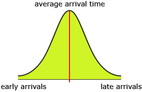
The normal curve arises because the outcomes of random situations will frequently be clustered around the mean with only a few outcomes far away from the mean. Again, consider students arriving for class. Most of the students arrive for class at about the same time. The further you are from the average time, the fewer students are arriving.
Now, this frequency distribution might not be true if your data is for only a few people in your class. But what if you had the class arrival times for the entire population of high school students in Canada or the world? Do you think that data will better approximate a normal distribution if the number of data values increased?