Lesson 3
Completion requirements
Created by IMSreader
1. Lesson 3
1.8. Explore 4
Module 4: Polynomials
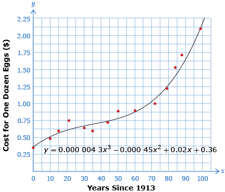
Consider the following data. The table shows the cost of one dozen eggs from 1913 to present day.
| Year Since 1913 | 0 | 10 | 15 | 22 | 30 | 35 | 44 | 50 | 60 | 72 | 79 | 84 | 88 | 99 |
| Cost of One Dozen Eggs ($) | 0.35 | 0.48 | 0.60 | 0.75 | 0.64 | 0.60 | 0.72 | 0.88 | 0.90 | 1.00 | 1.22 | 1.54 | 1.70 | 2.10 |

iStockphoto/Thinkstock
Draw a scatter plot of the data. Then compare your scatter plot with the following.
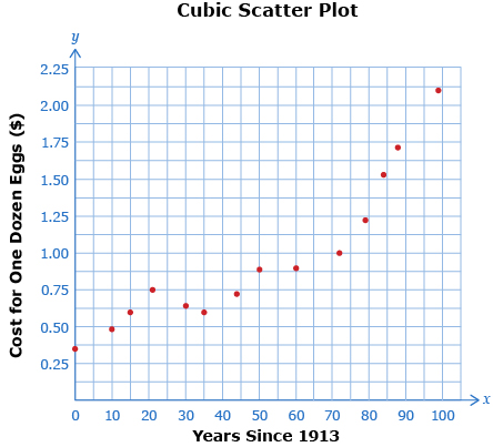
What do you notice? Is the data linear? quadratic? neither?
The data is neither linear nor quadratic and would best be modelled by a cubic function.
Use your graphing calculator to find the cubic regression equation (much like you have found the linear regression equations and quadratic regression equations).
The equation from your calculator (after some rounding) should be
y = 0.000 004 3x3 − 0.000 45x2 + 0.02x + 0.36
Plotting the cubic curve of best fit yields the following graph: