Lesson 3
1. Lesson 3
Module 4: Polynomials
Lesson 3: Modelling Data with a Curve of Best Fit
Focus
In Lesson 2 you were introduced to using linear regression to draw conclusions about data that exhibits a linear trend. What about data that does not have a linear trend? For example, what about the revenue data from the drama scenario introduced in Lesson 1?
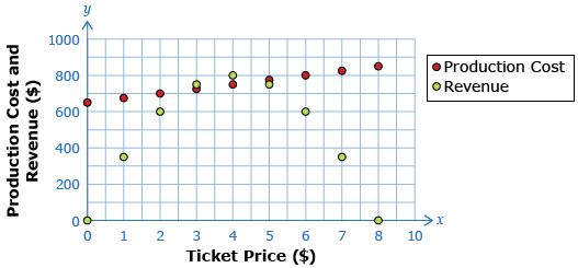
Data Source: PRINCIPLES OF MATHEMATICS 12 by Canavan-McGrath et al. Copyright Nelson Education Ltd. Reprinted with permission.
In this lesson you will learn about quadratic and cubic regressions and use those equations to model real-world problems.
Lesson Outcomes
At the end of this lesson you will be able to
- use technology to determine quadratic and cubic regression equations
- use a regression equation to answer questions in a real-world context
Lesson Question
You will investigate the following question: How can a curve of best fit be used to model problems?
Assessment
Your assessment may be based on a combination of the following tasks:
- completion of the Lesson 3 Assignment (Download the Lesson 3 Assignment and save it in your course folder now.)
- course folder submissions from Try This and Share activities
- work under Project Connection