Module 4 Summary
1. Module 4 Summary
Module 4 Summary

iStockphoto/Thinkstock
Polynomial functions can be used to model many real-world problems. In this module you
- sketched representative graphs of linear, quadratic, and cubic polynomial functions
- related characteristics of graphs of polynomial functions to the functions’ algebraic forms
- used technology to determine equations of lines and curves of best fit
- used regression equations to answer questions in real-world contexts
In the Module 4 Project you explored and analyzed shapes of polynomials found in our environment.
Following are some of the key ideas you learned in each lesson.
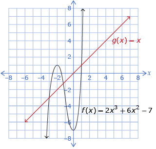
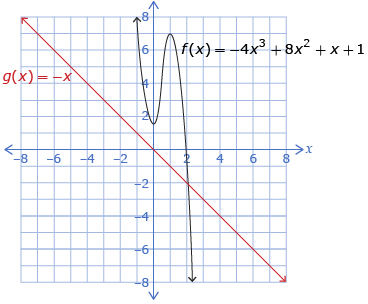
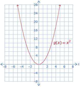
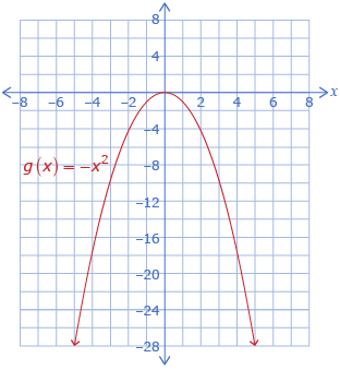
| Lesson 1 | The general shape of the graph of a polynomial function is determined by the type of function (linear, quadratic, cubic) and the sign of the leading coefficient.
Linear and Cubic, Positive Leading Coefficient
Linear and Cubic, Negative Leading Coefficient
Quadratic, Positive Leading Coefficient
Quadratic, Negative Leading Coefficient
|
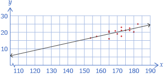
| Lesson 2 | Lines of best fit can be created for data that exhibits a linear trend.
|
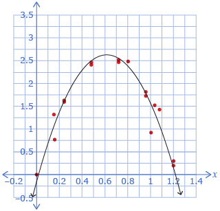
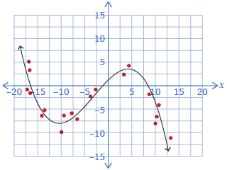
| Lesson 3 | Curves of best fit can be created for data that exhibits quadratic or cubic trends.
Quadratic Trend
Cubic Trend
|